2004 POSTS

JANUARY 2004

The mathematics of human thought

This year marks the 150th anniversary of the publication of the book that set the scene for the introduction of the computer a century later: George Boole’s The Laws of Thought, first published in 1854. The dramatic breakthrough that the book represented is reflected today in our use of the terms “boolean logic” or “boolean algebra” to mean the combination of ideas using the operations AND, OR, and NOT, and our use of the term “boolean search” to mean a database or Web search involving combinations of key words using AND, OR, and NOT. (The fact that we generally do not capitalize “boole” in those contexts indicates just how pervasive Boole’s influence has been.)

Boole’s book begins with these words:

The design of the following treatise is to investigate the fundamental laws of those operations of the mind by which reasoning is performed; to give expression to them in the symbolic language of a Calculus, and upon this foundation to establish the science of Logic and construct its method.

By the phrase “the symbolic language of a Calculus” Boole meant algebra. Not just the use of algebraic symbols like x, y, z, p, q, r to denote unknown words, phrases, or propositions. That much had been done by the logicians of ancient Greece. What Boole was talking about was using the entire apparatus of the high school algebra class, with operations such as addition and multiplication and the employment of methods to solve equations. Boole’s algebra required the formulation of a symbolic language of thought. Solving an equation in that language would not lead to a numerical answer; it would give the conclusion of a logical argument. His algebra was to be an algebra of thought.

Even today, in the twenty-first century, when we are familiar with computers—the “thinking machines” that are direct descendants of Boole’s logical algebra—it seems an audacious idea to write down algebraic equations that describe the way we think. What led Boole to propose such a thing, and why did he think it might be successful?

George Boole was born in England in 1815. Though the world was to regard him as a mathematician—indeed, as one of the most influential mathematicians of all time—he shared his interests between mathematics and psychology. Were he alive today, he would undoubtedly refer to himself as a cognitive scientist, a term that was first used in the early 1950s. He was largely self taught, and it may have been the absence of a teacher to lead him away from such a seemingly nonsensical idea that enabled him to seek to capture the patterns of thought by means of algebra. The mark of his genius is that he succeeded to such an extent.

Boole first published his algebra of thought in 1847 in a small pamphlet entitled The Mathematical Analysis of Logic. The simplest way to describe the contents of this pamphlet is to quote from the opening section.

They who are acquainted with the present state of the theory of Symbolic Algebra, are aware that the validity of the processes of analysis does not depend upon the interpretation of the symbols which are employed, but solely upon the laws of their combination. Every system of interpretation which does not affect the truth of the relations supposed, is equally admissible, and it is thus that the same processes may, under one scheme of interpretation, represent the solution of a question on the properties of number, under another, that of a geometrical problem, and under a third, that of a problem of dynamics or optics. … It is upon the foundation of this general principle, that I purpose to establish the Calculus of Logic …

It is worth reading through the above passage a second time. Boole made every word count.

As a result of his new algebra of logic, in 1849 Boole was appointed to the chair of mathematics at the newly founded University College, Cork. As soon as he had established residence in Ireland, he began work on a larger book about his new theory. He was particularly keen to ensure that his mathematics really did capture laws of mental activity, and to this end he spent a great deal of time reading psychological literature and familiarizing himself with what the philosophers had to say about mind and logic.

He used his own money and that of a friend to publish his second, more substantial book on his ideas in 1854. Its full title was An Investigation of the Laws of Thought on Which are Founded the Mathematical Theories of Logic and Probabilities. but it is generally referred to more simply as The Laws of Thought. By and large, the only substantial difference between the 1854 book and the earlier pamphlet of 1847 was the addition of his treatment of probability, using his new algebraic framework. The logic itself was largely unchanged.

Boole’s idea was to try to reduce logical thought to the solution of equations—a logical holy grail ever since the German mathematician Gottfried Leibniz had tried to do it in the 17th century. Leibniz attempted to develop an “algebra of concepts”, in which algebraic symbols had denoted concepts, such as big, red, man, woman, unicorn, but he had met with only limited success.

Boole wanted his algebra to encompass all of Aristotle’s insights into human reasoning (the famous Greek “All men are mortal” syllogisms) as well as the Stoics’ logic of propositions (what we now refer to as propositional calculus). He took his symbols x, y, z, etc. to denote arbitrary collections of objects. For example, the collection of all men, the collection of all mortals, the collection of all bankers, or the collection of all natural numbers. He then showed how to do algebra with symbols that denote collections—to write down and solve equations—in a way that corresponds to performing logical deductions.

In order to be able to write down and solve algebraic equations involving collections, Boole had to define what it meant to add and to multiply two collections. Since his algebra was intended to capture some of the patterns of logical thought, his definitions of addition and multiplication had to correspond to some basic thought processes. Moreover, it would be easier to do algebra if he could define addition and multiplication in such a way that they had many of the familiar properties of addition and multiplication of numbers, making his new algebra of thought similar to the algebra everyone was used to.

Here is what he did. Given collections x and y, Boole denoted the collection of objects common to both x and y by xy. For example, if x is the collection of all Germans and y is the collection of all sailors, then xy is the collection of all German sailors.

Boole’s definition of addition was more complicated than it needed to be, so other mathematicians of the time modified it to the following simple idea: x + y is the collection of objects that are in either x or y or both. For example, if x is the collection of all red pens and y is the collection of all blue pens, then x + y is the collection of all pens that are either red or blue.

With these definitions of multiplication and addition, Boole’s system had the following properties:

x + y = y + x

xy = yx

x + (y + z) = (x + y) + z

x(yz) = (xy)z

x(y + z) = xy + xz

These equations should look familiar for ordinary arithmetic, where the letters denote numbers. They are the two commutative laws, the two associative laws, and the distributive law. Because of the similarities between Boole’s algebra of collections and ordinary arithmetic, Boole was able to perform calculations in his system, i.e., algebraic manipulations such as solving equations. However, solving an equation in Boole’s system corresponds not to arithmetic but to logical reasoning about … well, about whatever the symbols are taken to mean—men, women, unicorns, what to prepare for dinner, etc. True, solving Boolean equations is not necessarily the best way to make a human decision. But the point was that patterns of logical thought could be represented by means of algebra. How far that would get you in real life was a question for later generations to take up.

There are further similarities between Boole’s system and ordinary algebra. For instance, in ordinary arithmetic the number 0 is special: adding 0 to any number leaves the number unchanged. In order for his algebra to work, Boole also needed a zero. He obtained it by taking 0 to be the empty collection.

One advantage of having a 0 is that it provides a way to write down an algebraic equation saying that various things do not exist. For example, in Boole’s algebra we can express the fact that unicorns do not exist by letting x be the collection of all unicorns and writing down the equation x = 0.

With 0 defined as the empty collection, the symbol 0 has the same special properties in Boole’s algebra of collections as it does in ordinary algebra:

x + 0 = x

x0 = 0

for any collection x.

Although Boole’s algebra had many of the properties of ordinary algebra, it was not exactly the same. Boole really did have to work with a strange, new kind of algebra. For instance, in Boole’s algebra, the following two equations are true:

x + x = x

xx = x

These equations are certainly not true for ordinary arithmetic.

Incidentally, the axiomatic system that today’s mathematicians refer to as a “boolean algebra” is not due to Boole. Rather, it was developed by other mathematicians who built on Boole’s original work.

By reducing reasoning to doing algebra, Boole opened up the possibility of building a reasoning machine. Even today, it is hard to imagine any kind of mechanical or (these days) electronic machine being able to reason the way humans do about, say, local politics. What can a machine possible know about local government? On the other hand, even in Boole’s day it seemed perfectly possible to construct a machine that could manipulate algebraic symbols according to some general rules.

Indeed, the rules Boole presented for manipulating algebraic expressions and for solving equations in his system were sufficiently mechanical that the English logician W. S. Jevons was able to use them to build a mechanical reasoning machine which he demonstrated to the Royal Society in 1870. Not surprisingly, given the prevailing technology at the time, Jevons’ device looked for all the world like an old style mechanical cash register. But for all its antiquated appearance, as an implementation of logic it was a stunning early ancestor of the modern electronic computer.

Today’s electronic computer is, at heart, just an implementation in silicon of Boole’s algebra of thought, with streams of electrons performing Boole’s algebraic operations. The OR gates and AND gates you can read about in books that describe how computers work correspond directly to Boole’s algebraic operations of addition and multiplication. In last month’s column I described how the mathematician John von Neumann played a key role in the the design of one of the first electronic computers in the early 1950s. It was the theoretical work of George Boole a century earlier that prepared the foundations upon which von Neumann and this colleagues helped usher in today’s computer era.

NOTE: This months’ column is abridged from my book Goodbye Descartes: The End of Logic and the Search for a New Cosmology of the Mind, published by John Wiley in 1997. For more on George Boole, and the development of logic and its role in the invention of the modern computer, consult that book.
For more in-depth coverage of the use of language in mathematics, but still at an elementary level, see my book Sets, Functions, and Logic, the Third (completely revised) Edition of which has just been published by Chapman and Hall.

Devlin’s Angle is updated at the beginning of each month.

Mathematician Keith Devlin ( devlin@csli.stanford.edu) is the Executive Director of the Center for the Study of Language and Information at Stanford University and “The Math Guy” on NPR’s Weekend Edition. His most recent book is The Millennium Problems: The Seven Greatest Unsolved Mathematical Puzzles of Our Time, published by Basic Books (hardback 2002, paperback 2003).

FEBRUARY 2004

The Archimedes Cattle Problem

In the third century BC, the famous Greek mathematician Archimedes issued a challenge to the Alexandrian mathematicians, headed by Eratosthenes. Written in the form of an epigram, Archimedes’s challenge begins thus:

“Compute, o friend, the number of oxen of the Sun, giving thy mind thereto, if thou has a share of wisdom.”

He then goes on to describe, in wonderfully poetic language, a certain herd of cattle, consisting of four types, with bulls and cows of each type. The number of cattle in each of the eight categories is not given, but these numbers are related by nine simple conditions which Archimedes spells out. For example, one of these conditions is that the number of white bulls is equal to the number of yellow bulls plus five-sixths of the number of black bulls. The problem is to determine the number of cattle of each category, and thence the size of the herd. (Actually, what is required is the smallest possible number, since the nine conditions do not imply a unique answer. I’ll give the actual problem in a moment.)

In his epigram, Archimedes goes on to say that anyone who solves the problem would be “not unknowing nor unskilled in numbers, but still not yet to be numbered among the wise.” Nothing could be more apt, since there was to elapse 2,000 years before a computer finally found the solution. Clearly Archimedes had a mischievous streak in addition to his principles, and was trying to pull a fast one on his Alexandrian rivals.

In 1880, a German mathematician called Amthor showed that the total number of cattle in Archimedes herd had to be a number with 206,545 digits, beginning with 7766. Not surprisingly, Amthor gave up at that point. Over the next 85 years, a further 40 digits were worked out. But it was not until 1965 when mathematicians at the University of Waterloo in Canada finally found the complete solution. It took over seven and a half hours of computation on an IBM 7040 computer. Unfortunately, no one thought to keep the printout of the answer! The world had to wait until the problem was solved a second time using a Cray-1 computer in 1981 for a published printout. It took the Cray just 10 minutes to crack it. But after 2,000 years I think Archimedes has to have the last laugh.

So what is Archimedes’ Cattle Problem?

Archimedes asks you to imagine a certain herd of cattle consisting of both cows and bulls, each of which may be white, black, yellow, or dappled. The numbers of each category of cattle are connected by various, simple conditions. To give these, let W denote the number of white bulls, w the number of white cows, B the number of black bulls, b the number of black cows, with Y, y and D, d playing analogous roles for the other colors. Using Archimedes’ method of writing fractions (that is, utilizing only simple reciprocals), the fist seven conditions which these various numbers have to satisfy are:

(1) W = (1/2 + 1/3)B + y

(2) B = (1/4 + 1/5)D + Y

(3) D = (1/6 + 1/7)W + Y

(4) w = (1/3 + 1/4)(B + b)

(5) b = (1/4 + 1/5)(D + d)

(6) d = (1/5 + 1/6)(Y + y)

(7) y = (1/6 + 1/7)(W + w)

The two remaining conditions are:

(8) W + B is a perfect square

(9) Y + D is a triangular number.

[A triangular number is one that is equal to a number of balls that may be arranged to form a triangle, which is the same as saying that the number must be of the form n(n+1)/2 for some n.]

The problem is to determine the size of the eight unknowns, and thus the size of the herd. More precisely, the aim is to find the least solution, since the conditions admit more than one solution. If conditions (8) and (9) are dropped, the problem is relatively easy. The smallest herd consists of 50,389,082 cattle. The additional two conditions make the problem considerably harder. It has been claimed that the first complete solution was worked out by the Hillsboro (Illinois) Mathematics Club between 1889 and 1893, although no copy of their solution has ever been found, and there is some evidence to suggest that what they in fact did was work out some of the digits of the 206,545 digit solution and provide an algorithm for the computation of the remainder.

In 1965, H. C. Williams, R. A. German, and C. R. Zarnke at the University of Waterloo in Canada used an IBM 7040 computer to crack the problem once and for all. The final solution occupied 42 sheets of print-out. In 1981, Harry Nelson repeated the calculation using a Cray-1. This machine took a mere 10 minutes to come up with the answer. Reduced to fit 12 pages of print-out on a single journal page, the solution was published in the Journal of Recreational Mathematics 13 (1981), pp.162-176.

The Math Guy on NPR radio

I often get emails from math instructors who want to locate one of my “Math Guy” conversations with host Scott Simon on NPR’s Weekend Edition. The Math Guy slot has been on the air since 1996 (although the name “Math Guy” did not come until later), on an irregular basis, and to date there have been 34 such segments. Since 1998, NPR has made the sound files available on its website. For a complete list, with links, go to http://profkeithdevlin.com/MathGuy.html.

Devlin’s Angle is updated at the beginning of each month.

Mathematician Keith Devlin (Email: devlin@csli.stanford.edu) is the Executive Director of the Center for the Study of Language and Information at Stanford University and “The Math Guy” on NPR’s Weekend Edition. His most recent book is The Millennium Problems: The Seven Greatest Unsolved Mathematical Puzzles of Our Time, published by Basic Books (hardback 2002, paperback 2003).

MARCH 2004

A Year of Anniversaries

The year 2004 sees an unusually large number of anniversaries of major advances in mathematics. I began the year with my January column devoted to one of those anniversaries: It is exactly 150 years since the publication in 1854 of George Boole’s major work The Laws of Thought. But that merely scratched the surface of this bumper anniversary year.

350 years: In an exchange of five letters in 1654, Pierre De Fermat and Blaise Pascal founded modern probability theory.

250 years: In 1754, Joseph-Louis Lagrange made important discoveries about the tautochrone, which in due course would contribute substantially to the new subject of the calculus of variations.

200 years: In 1804, Wilhelm Bessel published a paper on the orbit of Halley’s comet, based on observations by Thomas Harriot 200 years earlier.

150 years: Three major developments took place in 1854. In addition to Boole’s publication of The Laws of Thought in England, Arthur Cayley (also in England) made the first attempt to define an abstract group, while in Germany Bernhard Riemann completed his Habilitation. In his dissertation, Riemann studied the representability of functions by trigonometric series and gave the conditions for a function to have an integral (what we now call “Riemann integrability”). In a lecture titled On the hypotheses that lie at the foundations of geometry, given on 10 June 1854, he defined an n-dimensional space and gave a definition of what is today called a “Riemannian space”.

100 years: In 1904, Henri Poincare came within a whisker of discovering relativity theory. In an address to the International Congress of Arts and Science in St Louis, he remarked that observers in different frames will have clocks which will “… mark what one may call the local time. … as demanded by the relativity principle the observer cannot know whether he is at rest or in absolute motion.” Unfortunately, he never took the next step—the full Principal of Special Relativity—leaving the field open for Albert Einstein to make that important leap forward and claim the credit the following year.

I’ll take a look at some of these major advances in future columns. This month, I want to look in depth at the oldest one: the Fermat-Pascal correspondence that established modern probability theory. My account is taken from my book The Language of Mathematics.

Figuring the odds

The first step toward a theory of probability came when a sixteenth century Italian physician—and keen gambler—called Girolamo Cardano described how to give numerical values to the possible outcomes of the roll of dice. He wrote up his observations in a book titled Book on Games of Chance, which he published in 1525.

Suppose you roll a die, said Cardano. Assuming the die is “honest”, there is an equal chance that it will land with any of the numbers 1 to 6 on top. Thus, the chance that each of the numbers 1 to 6 ends face up is 1 in 6, or 1/6. Today, we use the word “probability” for this numerical value: We say that the probability that the number 5, say, is thrown is 1/6.

Going a step further, Cardano reasoned that the probability of throwing either a 1 or a 2 must be 2/6, or 1/3, since the desired outcome is one of two possibilities from a total of six.

Going further still—though not quite far enough to make a real scientific breakthrough—Cardano calculated the probabilities of certain outcomes when the die is thrown repeatedly, or when two dice are thrown at once.

For instance, what is the probability of throwing, say, a 6 twice in two successive rolls of a die? Cardano reasoned that it must be 1/6 times 1/6, that is, 1/36. You multiply the two probabilities since each of the six possible outcomes on the first roll can occur with each of the six possible outcomes on the second roll, that is, 36 possible combinations in all. Likewise, the probability of throwing, say, a 1 or a 2 twice in two successive rolls is 1/3 times 1/3, namely 1/9.

What is the probability that, when two dice are thrown, the two numbers showing face up will add up to, say, 5? Here is how Cardano analyzed that problem. For each die, there are six possible outcomes. So there are 36 (= 6 x 6) possible outcomes when the two dice are thrown: each of the six possible outcomes for one of the two dice can occur with each of the six possible outcomes for the other. How many of these outcomes sum to 5? List them all: 1 and 4, 2 and 3, 3 and 2, 4 and 1. That’s four possibilities altogether. So of the 36 possible outcomes, 4 give a sum of 5. So, the probability of a sum of 5 is 4/36, that is, 1/9.

Cardano’s analysis provided just enough for a prudent gambler to be able to bet wisely on the throw of the dice—or perhaps be wise enough not to play at all. But Cardano stopped just short of the key step that leads to the modern theory of probability. So too did the great Italian physicist Galileo, who rediscovered much of Cardano’s analysis early in the seventeenth century, at the request of his patron, the Grand Duke of Tuscany, who wanted to improve his performance at the gambling tables. What stopped both Cardano and Galileo was that they did not look to see if there was a way to use their numbers—their probabilities—to predict the future.

That key step was left to the two French mathematicians Blaise Pascal and Pierre de Fermat. In 1654, the two exchanged a series of five letters (the last was dated 27 October) that most people today agree was the beginning of the modern theory of probability. Though their analysis was phrased in terms of one specific problem about gambling, Pascal and Fermat developed a general theory that could be applied in a wide variety of circumstances, to predict the likely outcomes of various courses of events.

The problem that Pascal and Fermat examined in their letters had been around for at least two hundred years: How do two gamblers split the pot if their game is interrupted part way through? For instance, suppose the two gamblers are playing a best-out-of-five dice game. In the middle of the game, with one player leading two to one, they have to abandon the game. How should they divide the pot?

If the game were tied, there wouldn’t be a problem. They could simply split the pot in half. But in the case being examined, the game is not tied. To be fair, they need to divide the pot to reflect the two-to-one advantage that one player has over the other. They somehow have to figure out what would most likely have happened had the game been allowed to continue. In other words, they have to be able to look into the future—or in this case, a hypothetical future that never came to pass.

The problem of the unfinished game seems to have first appeared in the fifteenth century, when it was posed by Luca Paccioli, the monk who taught Leonardo de Vinci mathematics. It was brought to Pascal’s attention by Chevalier de Mere, a French nobleman with a taste for both gambling and mathematics. Unable to resolve the puzzle on his own, Pascal asked Fermat—widely regarded as the most powerful mathematical intellect of the time—for his help.

In their letters, Pascal and Fermat not only solved the puzzle of the unfinished game, but in so doing they established the foundations of modern probability theory.

To arrive at an answer to Pacciola’s puzzle, Pascal and Fermat examined all the possible ways the game could have continued, and observed which player won in each case. For instance, in the case of the best-of-five dice game that is stopped after the third round with one player in the lead by two to one, there are four possible ways the game can be completed. Of those four, three are won by the player in the lead after the third round. So the two players should split the pot with 3/4 going to the person in the lead and 1/4 going to the other.

Alhough Pascal and Fermat developed the theory of probability collaboratively, through their correspondence—the two men never met—they each approached the problem in different ways. Fermat preferred the algebraic techniques that he used to such devastating effect in number theory. Pascal, on the other hand, looked for geometric order beneath the patterns of chance. That random events do indeed exhibit geometric patterns is illustrated in dramatic fashion by what is now called Pascal’s triangle, shown here.

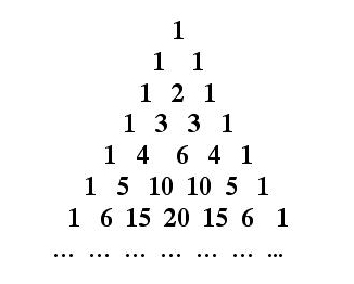
The symmetrical array of numbers shown in the figure is constructed according to the following simple procedure.

At the top, start with a 1.

On the line beneath, put two 1s.

On the line beneath that, put a 1 at each end, and in the middle the sum of the two numbers above and to each side, namely 1 + 1 = 2.

On line four, put a 1 at each end, and at each point midway between two adjacent numbers on line three put the sum of those numbers. Thus, in the second place you put 1 + 2 = 3 and in the third place you put 2 + 1 = 3.

On line five, put a 1 at each end, and at each point midway between two adjacent numbers on line four put the sum of those numbers. Thus, in the second place you put 1 + 3 = 4, in the third place you put 3 + 3 = 6, and in the fourth place you put 3 + 1 = 4.

By continuing in this fashion as far as you want, you generate Pascal’s triangle. The patterns of numbers in each row occur frequently in probability computations—Pascal’s triangle exhibits a geometric pattern in the world of chance.

For example, suppose that when a married couple have a child, there is an equal chance of the baby being male or female. (This is actually not quite accurate, but it’s close.) What is the probability that a couple with two children will have two boys? A boy and a girl? Two girls? The answers are, respectively, 1/4, 1/2, and 1/4. Here’s why. The first child can be male or female, and likewise the second. So we have the following four possibilities (in order of birth in each case): boy-boy, boy-girl, girl-boy, girl-girl. Each of these four possibilities is equally likely, so there is a 1-in-4 probability that the couple will have two boys, a 2-in-4 (i.e., 1/2) probability of having one of each gender, and a 1-in-4 probability of having two girls.

Here is where Pascal’s triangle comes in. The third line of the triangle reads 1 2 1. The sum of these three numbers is 4. Dividing each number on the row by the sum 4, we get (in order): 1/4, 2/4 (= 1/2), 1/4, the three probabilities for the different kinds of family.

Suppose the couple decide to have three children. What are the probabilities that they have three boys? Two boys and a girl? Two girls and a boy? Three girls? The fourth row of Pascal’s triangle gives the answers. The row reads: 1 3 3 1. These numbers sum to 8. The different probabilities are, respectively: 1/8, 3/8, 3/8, 1/8.

Similarly, if the couple has four children, the various possible gender combinations have probabilities 1/16, 4/16, 6/16, 4/16, 1/16. Simplifying these fractions, the probabilities read: 1/16, 1/4, 3/8, 1/4, 1/16.

In general, whenever there is an event where the individual outcomes can occur with equal probability, Pascal’s triangle gives the probabilities of the different possible combinations that can arise when the event is repeated a fixed number of times. If the event is repeated N times, you look at the N+1’st row of the triangle, and the numbers in the row give the numbers of different ways each particular combination can arise. Dividing the row numbers by the sum of the numbers in the row then gives the probabilities.

Since Pascal’s triangle can be generated by a simple geometric procedure, this method shows that there is geometric structure beneath questions of probability. It’s discovery was a magnificent achievement.

Addendum to last month’s column

Last month, I discussed the Archimedes cattle problem, oberving that, in 1981, Harry Nelson solved the problem in ten minutes on a Cray-1 supercomputer. Stan Wagon wrote to point out that algorithms have improved since then. According to Wagon, a good modern laptop can solve the problem in about a second using Mathematica. A section is devoted to this in Wagon and Bressoud’s book A Course In Computational Number Theory. Section 7.5 of the book is titled “Archimedes and the Sun God’s Cattle”. Solving the basic equation (a Pell equation) involved takes 0.01 seconds, but then you have to go through a While loop to get the right solution, and that takes 0.07 seconds.

Wagon also notes that some ideas of Ilan Vardi allow an even faster approach that requires almost no computation. Vardi’s work is detailed in his paper Archimedes’ Cattle Problem,American Mathematical Monthly 105 (1998) 305-319.

Devlin’s Angle is updated at the beginning of each month.

Mathematician Keith Devlin (Email: devlin@csli.stanford.edu) is the Executive Director of the Center for the Study of Language and Information at Stanford University and “The Math Guy” on NPR’s Weekend Edition. For a complete list of Math Guy segments, with links, go to http://www- csli.stanford.edu/~devlin/MathGuy.html

Devlin’s most recent book is The Millennium Problems: The Seven Greatest Unsolved Mathematical Puzzles of Our Time, published by Basic Books (hardback 2002, paperback 2003).

APRIL 2004

The Abel Prize Awarded: The Mathematicians’ Nobel

The Abel Prize, established by the Norwegian government in 2001 as an annual “Nobel Prize for Mathematics” and first awarded last year, will go this year to Professor Isadore Singer, 80, of MIT and Sir Michael Atiyah, 75, who has held an honorary position at the University of Edinburgh since he retired from Cambridge University a few years ago.

The prize is being given for the work that led to the names Atiyah and Singer being forever linked in the field of mathematics: the “Atiyah-Singer Index Theorem”, which they formulated and proved in a series of papers they published in the early 1960s. The Index Theorem provides a bridge between pure mathematics (differential geometry, topology, and analysis) and theoretical physics (quantum field theory) that has led to advances in both fields.

The Norwegian Academy of Science, which oversees and manages the new prize, referred to the Index Theorem as “one of the great landmarks of 20th century mathematics”. In fact, it is no exaggeration to say that the result changed the landscape of mathematics. Atiyah, who trained as an algebraic geometer and topologist, and Singer, who came from analysis, worked on ramifications of the theorem for twenty years.

Sir Michael, quoted in an article in Britain’s Daily Telegraph newspaper (March 26) commented: “the Index Theorem provides a Trojan horse that mathematicians have used to get into physics and vice versa. When we first did it, we had no inkling that this would follow.”

Singer, speaking to BBC News (March 26), said: “I am delighted to win this prize with Sir Michael. The work we did broke barriers between different branches of mathematics and that’s probably its most important aspect. … It has also had serious applications in theoretical physics.” Referring to the creation of the Abel Prize, he added “I appreciate the attention mathematics will be getting. It’s well-deserved because mathematics is so basic to science and engineering.”

Atiyah and Singer will receive their award from Norway’s King Harald at a ceremony in Oslo on May 25.

The prize amount is 6 million Norwegian Kroner, currently about $875,000. The award of the first Abel Prize, made in 2003 with relatively little fanfair outside of Scandinavia, went to the French mathematician Jean-Pierre Serre for his work in algebraic geometry and number theory.

The Abel Prize

There is no Nobel Prize for mathematics, but many mathematicians have won the prize, most commonly for physics but occasionally for economics, and in one case for literature. For instance, when mathematician John Nash won a Nobel Prize in 1994, it was for a result that had a major impact in economics. (Nash’s achievement was celebrated in director Ron Howard’s 2002 movie A Beautiful Mind, starring Russell Crowe.)

The Abel Prize is intended to give the mathematicians their own equivalent of a Nobel Prize. Such an award was first proposed in 1902 by King Oscar II of Sweden and Norway, just a year after the award of the first Nobel Prizes. However, plans were dropped as the union between the two countries was dissolved in 1905. As a result, mathematics has never had an international prize of the same dimensions and importance as the Nobel Prize.

Plans for an Abel Prize were revived in 2000, and in 2001 the Norwegian Government granted NOK 200 million (about $22 million) to create the new award. Niels Henrik Abel (1802-1829), after whom the prize is named, was a leading 19th-century Norwegian mathematician whose work in algebra has had lasting impact despite Abel’s early death aged just 26. Today, every mathematics undergraduate encounters Abel’s name in connection with commutative groups, which are more commonly known as “abelian groups” (the lack of capitalization being a tacit acknowledgement of the degree to which his name has been institutionalized).

As it happens, Abel’s own field of group theory plays a role in the Atiyah-Singer Index Theorem, but this is not a condition for the award of the Abel Prize.

The Abel Prize is awarded annually, and is intended to present the field of mathematics with a prize at the highest level. Laureates are appointed by an independent committee of international mathematicians.

As a result of Norway’s action, made in part to celebrate the 200th anniversary of Abel’s birth in 2002, mathematicians now too have an award equivalent to the Nobel Prize. The question is, will the new prize achieve the international luster of a real Nobel? The Nobel Prize in Economics (as it is popularly, but incorrectly, called) achieved that status after it was introduced in 1968, but in that case the Bank of Sweden, which created the award, attached the magic name Nobel to it. (See later.) One could hardly expect Norway to name their prize after a famous Swede, especially when they have Abel to recognize.

Mathematics and the Nobel Prize

Alfred Nobel (1833-1896) made his fortune through the manufacture of explosives. He was born in Sweden, grew up in Russia, studied chemistry and technology in France and the US, and built up companies in several countries all over the world. In his will, Nobel designated the establishment of annual prizes to be given in five areas: Physics, Chemistry, Physiology or Medicine, Literature, and Peace. The prizes are intended to reward specific discoveries or breakthroughs, and the impact of these on the discipline. The first prizes were awarded in 1901. In 1968, a sixth prize was added, in Economics, donated by the Bank of Sweden to celebrate its tercentenary. Strictly speaking, it is not a Nobel Prize but “the Prize in Economic Sciences in Memory of Alfred Nobel.” The Royal Swedish Academy of Sciences selects the prizewinners for physics, chemistry, medicine, literature, and economics, the Nobel Institute at the Karolinska Institute awards the prize in medicine, and the Norwegian Nobel Institute handles the Peace Prize. The monetary amount of each prize varies from year to year. In 2003 it was SEK10 million, about $1.3 million.

Although Nobel did not will a prize for mathematics, over the years many mathematicians have won a Nobel Prize. Taking a fairly generous interpretation for what constitutes being a mathematician, the mathematical Laureates are:

1902 Lorentz (Physics)
1904 Rayleigh (Physics)
1911 Wien (Physics)
1918 Planck (Physics)
1921 Einstein (Physics)
1922 Bohr (Physics)
1929 de Broglie (Physics)
1932 Heisenberg (Physics)
1933 Schroedinger (Physics)
1933 Dirac (Physics)
1945 Pauli (Physics)
1950 Russell (Literature)
1954 Born (Physics)
1962 Landau (Physics)
1963 Wigner (Physics)
1965 Schwinger (Physics)
1965 Feynman (Physics)
1969 Tinbergen (Economics)
1975 Kantorovich (Economics)
1983 Chandrasekhar (Physics)
1994 Selten (Economics)
1994 Nash (Economics)

Overall, a fairly good showing for mathematics. Still, this isn’t the same as having a prize for mathematics itself.

A number of theories have been put forward to explain the omission of mathematics from Nobel’s original list. The most colorful suggestion is that Nobel was miffed at mathematicians after discovering that his wife had had an affair with the Swedish mathematician Magnus Mittag-Leffler. Of all the theories, this is the easiest to dismiss, for the simple reason that Nobel never had a wife.

Another oft-repeated suggestion is that Nobel hated mathematics after doing poorly in it at school. It may or may not be true that Nobel wasn’t good at math, but there is no evidence to suggest that a negative high school experience in the math class led to a desire to get back at the mathematicians later in life by not giving them one of his prizes.

By far the most likely explanation, I think, is that he viewed mathematics as merely a tool used in the sciences and in engineering, not as a body of human intellectual achievement in its own right. He also did not single out biology, possibly likewise regarding it as just a tool for medicine, a not unreasonable view to have in the late 19th century.

The Fields Medal

The Fields Medal is often cited as being “the mathematical equivalent of the Nobel Prize.” The Field Medals were first proposed at the 1924 International Congress of Mathematicians in Toronto by Professor J.C. Fields, a Canadian mathematician who was the secretary of the Congress that year. He later donated funds to establish the medals. Fields wanted the awards to recognize both existing work and the promise of future achievement, as a result of which it was agreed to restrict the medals to mathematicians not over forty at the year of the Congress. Medals are awarded every four years, at the Congress, by its organizing body, the International Mathematical Union. Initially, up to two medals were awarded every four years; in 1966 it was agreed that, in light of the great expansion of mathematical research, up to four medals could be awarded at each Congress.

“Fields Medals” are more properly known by their official name, “International medals for outstanding discoveries in mathematics.” The medal is accompanied by a cash prize of CND$15,000.

Atiyah himself received a Fields Medal in 1966.

There are some unique characteristics of the Fields Medal that make it different from a Nobel Prize. First it is awarded only every fourth year. Second, it is given for mathematical work done before the recipient is 40 years of age. Third, the monetary prize that goes with the Fields Medal is considerably less than the Nobel Prize. Fourth, the Fields Medal does not come out of Scandinavia.

When the Norwegian Academy of Science decided to create a prize for mathematics in honor of Abel, they did so with the intention of rectifying what they saw as an omission on the part of Nobel.

The Abel Prize winners

Isadore M. Singer was born in 1924 in Detroit, and received his undergraduate degree from the University of Michigan in 1944. After obtaining his Ph.D. from the University of Chicago in 1950, he joined the faculty at the Massachusetts Institute of Technology (MIT). Singer has spent most of his professional life at MIT, where he is currently an Institute Professor. He is a member of the American Academy of Art and Sciences, the American Philosophical Society and the National Academy of Sciences (NAS). He served on the Council of NAS, the Governing Board of the National Research Council, and the White House Science Council.

Michael Francis Atiyah was born in 1929 in London. He got his B.A. and his doctorate from Trinity College, Cambridge. He spent the greatest part of his academic career at the Universities of Cambridge and Oxford. He was the driving force behind the creation of the Isaac Newton Institute for Mathematical Sciences in Cambridge and became its first director. He was elected a Fellow of the Royal Society in 1962 at the age of 32, and was the Society’s president from 1990 to 1995. He was knighted in 1983 (hence “Sir Michael”) and made a member of the Order of Merit in 1992.

Because of its technical and highly abstract nature of the Index Theorem, it isn’t possible to give a precise statement in a column such as this. The exact formulation requires a heady mix of K-theory, functional analysis, and global analysis. Not long after I got my Ph.D., I met Atiyah in Oxford, and rushed off to read up about his famous theorem. I soon gave up, having decided that life was too short and I had my own mathematical research career to work on.

The press announcement of the award released by the Norwegian Academy of Sciences tried to convey the essence of the result with these words:

“We describe the world by measuring quantities and forces that vary over time and space. The rules of nature are often expressed by formulas involving their rates of change, so-called differential equations. Such formulas may have an “index”, the number of solutions of the formulas minus the number of restrictions which they impose on the values of the quantities being computed. The index theorem calculated this number in terms of the geometry of the surrounding space. … The Atiyah-Singer Index Theorem was the culmination and crowning achievement of a more than 100-year old development of ideas, from Stokes’s theorem, which students learn in calculus classes, to sophisticated modern theories like Hodge’s theory of harmonic integrals and Hirzebruch’s signature theorem.”

Let’s try to get a bit closer to the real thing.

Start with a compact smooth manifold (without boundary) and an elliptic operator E on it. (E is a differential operator acting on smooth sections of a given vector bundle. Laplacians are examples of elliptic operators.) The property of being elliptic is expressed by a symbol s that can be seen as coming from the coefficients of the highest order part of E; s is a bundle section and required to be non-zero. (In the case of a Laplacian, s is a positive-definite quadratic form.) The index of E is defined as the difference between the dimension of the kernel of E and the dimension of the cokernel of E. The “index problem” is to compute the index of E using only the symbol s and topological information about the manifold and the vector bundle. This problem seems to have emerged in the late 1950s. The Atiyah-Singer Index Theorem is its solution.

Devlin’s Angle is updated at the beginning of each month.

Mathematician Keith Devlin (Email: devlin@csli.stanford.edu) is the Executive Director of the Center for the Study of Language and Information at Stanford University and “The Math Guy” on NPR’s Weekend Edition. For a complete list of Math Guy segments, with links, go to http://www- csli.stanford.edu/~devlin/MathGuy.html

Devlin’s most recent book is The Millennium Problems: The Seven Greatest Unsolved Mathematical Puzzles of Our Time, published by Basic Books (hardback 2002, paperback 2003).

MAY 2004

The best popular science essay ever

I became a “math popularizer” almost by accident. In 1983 I had an idea for an April Fools spoof in a national daily newspaper, where I would write a mathematics story that was so counter-intuitive that everyone would think it was a spoof, but the real spoof would be that the story was in fact true. (The story was based on the fact that an engineering company had manufactured a rotary drill that would drill a square hole. To see the mathematics behind this feat, see http://mathworld.wolfram.com/ ReuleauxTriangle.html.)

I wrote it up and sent it in to the science page editor at The Guardian newspaper in my then home country of Britain. A couple of days later the editor telephoned me. He explained to me why my piece would not work in a national newspaper, but went on to say that he liked my writing style, and would be interested in seeing other contributions from me. A few months later an engineer at Cray Research discovered a new record Mersenne prime number, and I wrote a 700 word piece describing the discovery. The editor published it, the reader response was good, and within a short while I found myself a newspaper “math columnist”, with a twice monthly column in the science section.

It wasn’t long before book publishers started to approach me with requests for popular expositions of mathematics. Quite unplanned, I had a second career. Over the years, I have found myself spending more of my time on what has come to be called “public education”, but it remains a very small part of my regular activities. Nevertheless, I have taken it seriously. I read as many popular science books and newspaper and magazine articles about science I can, and I study closely the way the different successful science writers and journalists go about their job.

An essential device in trying to convey mathematics or science to a lay audience is metaphor. The more basic and familiar the metaphor, the greater the audience the writer can reach. To my mind, the queen of the metaphor in science writing is K. C. Cole of the Los Angeles Times. K.C. (as she prefers to be called) has published several collections of her articles from the LA Times in book form, and I recommend them all to anyone who wants to try their hand at science writing for a lay audience.

My all time favorite K.C. Cole piece, which I would claim is the best short newspaper article about science ever, first appeared in her “Mind over Matter” column in the Times on May 11, 2000. (Here on the West Coast we don’t use the initials “LA”, since the New York Times is referred to by its full name.) Titled “Murmurs”, it was republished in K.C.’s book Mind Over Matter: Conversations with the Cosmos, published by Harcourt in 2000 (pp. 15-17). In exactly 700 words (the ideal target length for a newspaper column), using a string of brilliantly conceived everyday metaphors, K.C. succeeds in describing the birth and early development of the universe. Not just describing; she brings it to life. At the same time, she manages to convey the dedication and the excitement of the astrophysics community in their quest to piece together this remarkable story.

With K.C.’s permission, I am reprinting her entire article. There is no special occasion. I just felt this marvellous piece deserved a further spin. I have resisted the temptation to analyze the article paragraph by paragraph, although I have done so for myself and found it well worth the effort. You can dissect it for yourself.

Here then, is what I claim is the best short, lay exposition of science there has ever been.

Murmurs

by K. C. Cole

When the universe speaks, astronomers listen.

When it sings, they swoon.

That’s roughly what happened recently when a group of astronomers published the most detailed analysis yet of the cosmos’s primordial song: a low hum, deep in its throat, that preceded both atoms and stars.

It is a simple sound, like the mantra “Om.” But hidden within its harmonics are details of the universe’s shape, composition, and birth. So rich are these details that within hours of the paper’s publication, new interpretations of the data has already appeared on the Los Alamos web server for new astrophysical papers.

“It’s stirred up a hornet’s nest of interest,” said UCLA astronomer Ned Wright, who gave a talk to his colleagues on the paper—as did so many others—the very next week.

So what is all the fuss about? Why are astronomers churning out paper after paper on what looks to a layperson like a puzzling set of wiggly peaks—graphic depictions of the sound, based on hours of mathematical analysis?

Because there’s scientific gold in them there sinusoidal hills.

The peak and valleys paint a visual picture of the sound the newborn universe made when it was still wet behind the ears, a mere 300,000 years after its birth in a big bang. Nothing existed but pure light, sprinkled with a smattering of subatomic particles.

Nothing happened, either, except that this light and matter fluid, as physicists call it, sloshed in and out of gravity wells, compressing the liquid in some places and spreading it out in others. Like banging on the head of a drum, the compression of the “liquid light” as it fell into gravity wells set up the “sound waves” that cosmologist Charles Lineweaver has called “the oldest music in the universe.”

Then, suddenly, the sound fell silent. The universe had gotten cold enough that the particles, in effect, congealed, like salad dressing left in the fridge; the light separated and escaped, like the oil on top.

The rest is the history of the universe: The particles joined each other to form atoms, stars, and everything else, including people.

“The universe was very simple back then,” said Caltech’s Andrew Lange in one talk. “After that, we have atoms, chemistry, economics. Things go downhill very quickly.”

As for the light, or radiation, it still pervades all space. In fact, it’s part of the familiar “snow” that sometimes shows up on broadcast TV. But it’s more than just noise: When the particles congealed, they left an imprint on the light.

Like children going after cookies, the patterns of sloshing particles left their sticky fingerprints all over the sky.

The pattern of the sloshes tells you all you need to know about the very early universe: its shape, how much was made of matter, how much of something else.

The principal is familiar: Your child’s voice sounds like no one else’s because that resonant cavities within her throat create a unique voiceprint. The large, heavy wood of the cello creates a mellower sound than the high-strung violin. Just so, the sounds coming from the early universe depend directly on the density of matter, and the shape of the cosmos itself.

Astronomers can’t hear the sounds, of course. But they can read them on the walls of the universe like notes on a page. Compressed sounds gets hot and produces hot splotches, like a pressure cooker. Expanded area’s cool. Analyze the hot and cold patches and you get a picture of the sound: exactly how much falls on middle C or B-flat.

What they’ve seen so far is both exciting and troubling. The sound suggests that the universe is a tad too heavy with ordinary matter to agree with standard cosmological theories; it resonates more like an oboe than a flute. Something’s going on that can’t be explained. The answers will come as even more sensitive cosmic stethoscopes listen in over the next few years.

Lest you think these sounds are music only for astronomers’ ears, consider: The same wrinkles in space that created the gravity wells that gave it rise to the sound also blew up to form clusters, galaxies, stars, planets, us.

Even Hare Krishnas murmuring Om.

Devlin’s Angle is updated at the beginning of each month.

Mathematician Keith Devlin (Email: devlin@csli.stanford.edu) is the Executive Director of the Center for the Study of Language and Information at Stanford University and “The Math Guy” on NPR’s Weekend Edition. For a complete list of Math Guy segments, with links, go to http://www- csli.stanford.edu/~devlin/MathGuy.html

Devlin’s most recent book is The Millennium Problems: The Seven Greatest Unsolved Mathematical Puzzles of Our Time, published by Basic Books (hardback 2002, paperback 2003).

JUNE 2004

Good stories, pity they’re not true

The enormous success of Dan Brown’s novel The Da Vinci Code has introduced the famous Golden Ratio (henceforth GR) to a whole new audience. Regular readers of this column will surely be familiar with the story. The ancient Greeks believed that there is a rectangle that the human eye finds the most pleasing, and that its aspect ratio is the positive root of the quadratic equation

x² – x – 1 = 0

You are faced with this equation when you try to determine how to divide a line segment into two pieces such that the ratio of the whole line to the longer part is equal to the ratio of the longer part to the shorter. The answer is an irrational number whose decimal expansion begins 1.618.

Having found this number, the story continues, the Greeks then made extensive use of the magic number in their architecture, including the famous Parthenon building in Athens. Inspired by the Greeks, future generations of architects likewise based their designs of buildings on this wonderful ratio. Painters did not lag far behind. The great Leonardo Da Vinci is said to have used the Golden Ratio to proportion the human figures in his paintings—which is how the Golden Ratio finds its way into Dan Brown’s potboiler.

It’s a great story that tends to get better every time it’s told. Unfortunately, apart from the fact that Euclid did solve the line division problem in his book Elements, there’s not a shred of evidence to support any of these claims, and good reason to believe they are completely false, as University of Maine mathematician George Markowsky pointed out in his article “Misconceptions About the Golden Ratio”, published in the College Mathematics Journal in January 1992. But with such a wonderful story, which marries some decidedly accessible pure mathematics with aethestics, architecture, and painting—a high school math teacher’s dream if ever there were one—the facts have had little impact.

But being aware that few people will take note of what I say has never stopped me before. (I was, after all, a department chair in a college mathematics department for four years and a college dean for another eight.) So let’s try to separate the fact from the fiction.

First, what do we know for sure about the Golden Ratio? As mentioned above, Euclid showed how to calculate it, but his interest seemed more that of mathematics than visual aesthestics or architecture, for he gave it the decidedly unromantic name “extreme and mean ratio”. The term “Divine Proportion,” which is oten used to refer to GR, first appeared with the publication of the three volume work by that name by the 15th century mathematician Luca Pacioli. Calling GR “golden” is even more recent: 1835, in fact, in a book written by the mathematician Martin Ohm (whose physicist brother discovered Ohm’s law).

It is also true that the Golden Ratio is linked to the pentagram (five-pointed star), to the five Platonic solids, to fractal geometry, to certain crystal structures, and to Penrose tilings. So far so good.

The oft repeated claim (actually, all claims about GR are oft repeated) that the ratios of successive terms of the Fibonacci sequence tend to GR is also correct. The Fibonacci sequence, you may recall, is generated by starting with 0, 1 and repeatedly applying the rule that each new number is equal to the sum of the two previous numbers. So 0+1 = 1, 1+1 = 2, 1+2 = 3, 2+3 = 5, etc., giving the sequence 1, 1, 2, 3, 5, 8, 13, 21, 34, 55, 89, 144, 233, … The sequence of successive ratios of the numbers in this sequence, namely 1/1 = 1; 2/1 = 2; 3/2 = 1.5; 5/3 = 1.666… ; 8/5 = 1.6; 13/8 = 1.625; 21/13 = 1.615…; 34/21 = 1.619…; 55/34 = 1.6176…; 89/55 = 1.6181; …, does indeed tend to GR. As I’ll explain momentarily, this is a key part of the explanation of why the Fibonacci numbers keep appearing in flowers and plants—which they do.

For instance, if you count the number of petals in most flowers you will find that the answer is a Fibonacci number. For example, an iris has 3 petals, a primrose 5, a delphinium 8, ragwort 13, an aster 21, daisies 13, 21, or 34, and Michaelmas daisies 55 or 89 petals. All Fibonacci numbers.

Again, if you look at a sunflower, you will see a beautiful pattern of two spirals, one running clockwise, the other counterclockwise. Count those spirals, and for most sunflowers you will find that there are 21 or 34 running clockwise and 34 or 55 counterclockwise, respectively—all Fibonacci numbers. Less common are sunflowers with 55 and 89, with 89 and 144, and even 144 and 233 in one confirmed case. Other flowers exhibit the same phenomenon; the wildflower Black-Eyed Susan is a good example. Similarly, pine cones have 5 clockwise spirals and 8 counterclockwise spirals, and the pineapple has 8 clockwise spirals and 13 going counterclockwise.

Finally, if you take a close look at the way leaves are located on the stems of trees and plants, you will see that they are located on a spiral that winds around the stem. Starting at one leaf, count how many complete turns of the spiral it takes before you find a second leaf directly above the first. Let P be that number. Also count the number of leaves you encounter (excluding the first one itself). That gives you another number Q. The quotient P/Q is called the divergence of the plant. (The divergence is characteristic for any particular species.) If you calculate the divergence for different species of plants, you find that both the numerator and the denominator are usually Fibonacci numbers. In particular, 1/2, 1/3, 2/5, 3/8, 5/13, and 8/21 are all common divergence ratios. For instance, common grasses have a divergence of 1/2, sedges have 1/3, many fruit trees (including the apple) have a divergence of 2/5, plantains have 3/8, and leeks come in at 5/13.

Although many of these observations were made a hundred year or more ago, it was only recently that mathematicians and scientists were finally able to figure out what is going on. It’s a question of Nature being efficient.

For instance, in the case of leaves, each new leaf is added so that it least obscures the leaves already below and is least obscured by any future leaves above it. Hence the leaves spiral around the stem. For seeds in the seedhead of a flower, Nature wants to pack in as many seeds as possible, and the way to do this is to add new seeds in a spiral fashion.

As early as the 18th century, mathematicians suspected that a single angle of rotation can make all of this happen in the most efficient way: the Golden Ratio (measured in number of turns per leaf, etc.). However, it took a long time to put together all the pieces of the puzzle, with the final step coming in the early 1990s.

The worst kind of angle for efficient growth would be a rational number of turns, eg. 2 turns, or 1/2 a turn, or 3/8 of a turn, since they will soon lead to a complete cycle. Mathematically, a turn through an irrational part of a circle will never cycle, but in practical terms it could eventually come close. What angle will come least close to a cycle? Maximum efficiency will be achieved when the angle is “furthest away” from being a rational. But what exactly does that mean? The appropriate way (via s vis plant growth) to measure how far removed from being rational an irrational number is, is to look at its continued fraction expansion. For GR, this is:

Rational numbers have a finite continued fraction. That unending, constant sequence of 1’s in the continued fraction for GR says that, measured in terms of continued fractions, GR is the irrational number furthest removed from being rational. And that’s the mathematical reason why Nature favors GR as her growth ratio. The Fibonacci numbers appear because the number of leaves, spirals, etc. are whole numbers, and (because of the ratio limit property mentioned above) the Fibonacci numbers are the best whole number approximations to a GR growth.

For other examples of the appearance of the Golden Ratio in Nature, the growth of the Nautilus shell is governed by the Golden Ratio, as is the path followed by a Pergrine falcon when it swoops down to catch its pray. In these cases, the explanation is that the GR is closely related to the logarithmic spiral, the spiral that turns by a constant angle along its entire length, making it everywhere self-similar.

As the Nautilus grows, it has repeated need to enlarge its living quarters. Since the creature does not change shape, rather simply grows larger, the most efficient way to do this is for its shell to grow in the self-similar form of a logarithmic spiral.

The falcon must keep the prey in its sight all the time, but, although its eyes are razor sharp, they are fixed in its head, one on either side. So what the creature does is swivel its head to one side, by an angle of about 40^o, and fix the prey in one eye. Keeping its head fixed at that 40^o angle, the falcon then dives in a way that keep the prey in view in that one eye. The fixed angle of the head results in the bird following an equi-angular spiral path that converges on the prey.

So much for the good (i.e., true) stuff. Now for those many, many myths about GR that continue to do the rounds. The issue here is not whether you can find GR somewhere. If you look hard enough you will be able to find any (reasonably sized) number almost anywhere. The question is whether there is more to it than mere numerology. Is there a good scientific explanation to show why GR appears (as with the examples from Nature mentioned above), or is there definite evidence that, say, a particular artist made deliberate use of GR in his or her work? If not, all you have is an unsubstantiated belief. You may as well believe in fairies.

First of all, whether or not the ancient Greeks felt that the Golden Ratio was the most perfect proportion for a rectangle, many modern humans do not. Numerous tests have failed to show up any one rectangle that most observers prefer, and preferences are easily influenced by other factors. As to the Parthenon, all it takes is more than a cursory glance at all the photos on the Web that purport to show the Golden Ratio in the structure, to see that they do nothing of the kind. (Look carefully at where and how the superimposed rectangle—usually red or yellow—is drawn and ask yourself: why put it exactly there and why make the lines so thick?)

Another claim is that if you measure the distance from the tip of your head to the floor and divide that by the distance from your belly button to the floor, you get GR. But this nonsense. First of all, you won’t get exactly the number GR. You never can; GR is irrational, remember. But in the case of measuring the human body, there is a lot of variation. True, the answers will always be fairly close to 1.6. But there’s nothing special about 1.6. Why not say the answer is 1.603? Besides, there’s no reason to divide the human body by the navel. If you spend a half an hour or so taking measurements of various parts of the body and tabulating the results, you will find any number of pairs of figures whose ratio is close to 1.6, or 1.5, or whatever you want.

Then there is the claim that Leonardo Da Vinci believed the Golden Ratio is the ratio of the height to the width of a “perfect” human face and that he used GR in his Vitruvian Manpainting. While there is no concrete evidence against this belief, there is no evidence for it either, so once again the only reason to believe it is that you want to. The same is also true for the common claims that Boticelli used GR to proportion Venus in his famous painting The Birth of Venus and that Georges Seurat based his painting The Parade of a Circus on GR.

Painters who definitely did make use of GR include Paul Serusier, Juan Gris, and Giro Severini, all in the early 19th century, and Salvador Dali in the 20th, but all four seem to have been experimenting with GR for its own sake rather than for some intrinsic aesthetic reason. Also, the Cubists did organize an exhibition called “Section d’Or” in Paris in 1912, but the name was just that; none of the art shown involved the Golden Ratio.

Then there are the claims that the Egyptian Pyramids and some Egyptian tombs were constructed using the Golden Ratio. There is no evidence to support these claims. Likewise there is no evidence to support the claim that some stone tablets show the Babylonians knew about the Golden Ratio, and in fact there is good reason to conclude that it’s false.

Turning to more modern architecture, while it is true that the famous French architect Corbusier advocated and used the Golden Ratio in architecture, the claim that many modern buildings are based on Golden Rectangles, among them the General Secretariat building at the United Nations headquarters in New York, seems to have no foundation. By way of an aside, a small (and not at all scientific) survey I carried out myself a few months ago revealed that all architects polled knew about the GR, and all believed that other architects used the GR in their work, but none of them had ever used it themselves. Make whatever inference you wish.

Music too is not without its GR fans. Among the many claims are: that some Gregorian chants are based on the Golden Ratio, that Mozart used the Golden Ratio in some of his music, and that Bartok used GR in some of his music. All those claims are without any concrete support. Less clear cut is whether Debussy used the Golden Ratio in some of his music. Here the experts don’t agree on whether some GR patterns that can be discerned are intended or spurious.

Poetry too is not immune, but here there is a refreshing surprise in store for us. Whereas the claim that the Roman poet Vergil based the meter of his poem Aeneid on the Golden Ratio has no support, it really is true that some 12th Century Sanskrit poems have a meter based on the Fibonacci sequence (and hence related to the Golden Ratio).

I could go on, as there are many more examples, ranging from the sacred (eg. the dimensions of the Ark of the Covenant) to the profane (such as, predicting the behavior of the stock market), all of which, on close examination, turn out to be without any supporting evidence whatsoever. Despite the lack of evidence, however, and in some cases in the face of evidence to the contrary, each claim seems to attract its own band of devotees, who will not for a moment entertain the possibility that their cherished beliefs are not true. Consequently, not only is GR a very special number mathematically—all of its genuine appearances in mathematics and Nature show that—it also has enormous cultural significance as the number that most people have the greatest number of false beliefs about. Now there’s a GR fact that has plenty of supporting evidence.

For more details on the Golden Ratio, including evidence to support many of the claims I have made above, see the Markowsky article mentioned earlier, as well as the excellent book The Golden Ratio: The Story of PHI, the World’s Most Astonishing Number, by Mario Livio. Also worth a visit is Ron Knott’s excellent website Fibonacci Numbers and the Golden Section, at the University of Surrey in England.

Devlin’s Angle is updated at the beginning of each month.

Mathematician Keith Devlin ( devlin@csli.stanford.edu) is the Executive Director of the Center for the Study of Language and Information at Stanford University and The Math Guy on NPR’s Weekend Edition. Devlin’s most recent book is Sets, Functions, and Logic: an Introduction to Abstract Mathematics (Third Edition), published by Chapman and Hall in 2003.

JULY-AUGUST 2004

The Two Envelopes Paradox

I received a letter recently asking for me to “rule” on a debate two people were having about the notorious two envelopes paradox. Since my efforts to convince people of the correct resolution to the Monty Hall Problem inevitably generate a small avalanche of letters claiming I am completely wrong, I have in the past hesitated to tackle the much, much trickier envelopes puzzle. But the time has come, I think, to throw caution to the wind, and enter the fray.

Here, for those unfamiliar with the problem, is what it says.

You are taking part in a game show. The host offers you two envelopes, each containing a check. You may choose one, keeping the money it contains. She tells you that one envelope contains exactly twice as much as the other, but does not tell you which is which.

Since you have no way of knowing which envelope contains the larger sum, you pick one at random. The host asks you to open the envelope. You do so and take out a check for $40,000.

Here is where things get interesting, especially for contestants who know some mathematics.

The host now says you have a chance to change your mind and choose the other envelope. If you don’t know anything about probability theory, particularly expectations, you probably say to yourself, the odds are fifty-fifty that you have chosen the larger sum, so you may as well stick with your first choice. (And you’d be right. But I’ll come back to this in a moment.)

On the other hand, if you know a bit (though not too much) about probability theory, you may well try to compute the expected gain due to swapping. The chances are you would argue as follows. The other envelope contains either $20,000 or $80,000, each with probability .5. Hence the expected gain of swapping is

[0.5 x 20,000] + [0.5 x 80,000] – 40,000 = 10,000

That’s an expected gain of $10,000. So you swap.

But wait a minute. There’s nothing special about the actual monetary amounts here, provided one envelope contains twice as much as the other. Suppose you opened one envelope and found $M. Then you would calculate your expected gain from swapping to be

[0.5 x M/2] + [0.5 x 2M] – M = M/4

and since M/4 is greater than zero you would swap. Right?

Okay, let’s take this line of reasoning a bit further. If it doesn’t matter what M is, then you don’t actually need to open the envelope at all. Whatever is in the envelope you would choose to swap. Still with me?

Well, if you don’t open the envelope, then you might as well choose the other envelope in the first place. And having swapped envelopes, you can repeat the same calculation again and again, swapping envelopes back and forward ad-infinitum. There is no limit to the cumulative expected gain you can obtain. But this is absurd.

And there’s the paradox. What is wrong with the computation of the expected gain from swapping?

The answer is everything. The above computation is meaningless—which is why it leads so easily to a nonsensical outcome. If you want to apply probability theory, you are free to do so, but you need to do it correctly. And that means working with actual probabilities, taking care to distinguish between prior and posterior probabilities. Let’s take a closer look.

As with the Monty Hall Problem, if you really want to analyze the situation, you have to start by looking at the way the scenario was set up.

Let L denote the lower dollar value of the two checks. The other check thus has value 2L. Let P(L) be the prior probability distribution for the choice the host makes for the lower value in the envelopes. (This will affect the entire game. Of course, we don’t know anything about this distribution. But we can see how it affects the outcome of the game. Read on.

When you make your choice (C) during the game, you choose either the envelope containing the lower value (C=lower) or the one that contains the higher (C=higher). As the amounts are hidden from you, you choose entirely at random, with equal probabilities for the two options, so

P(C=lower) = P(C=higher) = 0.5

During the game, the value (V) of the content of the chosen envelope is revealed to be a certain value M. Given this information, what is the posterior probability that the chosen envelope contains the higher or lower value? That is, what is P(C|V=M), the probability that you chose the envelope containing the lower/higher value, given you now know what V is? This is the probability you need in order to compute any expected gain. The correct expected gain calculation is:

(2M)P(C=lower|V=M)+(M/2)P(C=higher|V=M) – M

The paradox above arose because you assumed that

P(C=lower|V=M) = P(C=higher|V=M) = 0.5

Let’s see why this cannot be the case. (In what follows, remember that L, V, C are variables and M is a numerical constant.)

By Bayes’ Theorem:

P(C|V=M) = P(V=M|C)P(C)/P(V=M) . . . (1)

Taking the first of the two cases, where you choose the lower value (V=L), we have

P(V=M|C=lower) = P(L=M)

The second of the two cases, where the chosen envelope contains double the lower value, is

P(V=M|C=higher) = P(L=M/2)

Substituting each of these two identities in to (1) gives

P(C=lower|V=M) = P(C=lower)P(L=M)/P(V=M) . . . (2)

and

P(C=higher|V=M) = P(C=higher)P(L=M/2)/P(V=M) . . . (3)

From (2), P(C=lower|V=M) is the same as P(C=lower) only if P(L=M) is the same as P(V=M). If it is not then in the calculations of expected gain you have used the incorrect probability. Specifically, you have used the prior probability, P(C=lower)=0.5, of choosing the lower value, rather than the posterior probability P(C=lower|V). The same argument works for P(C=higher|V), starting from (3).

Under what circumstances could we have P(L=M) = P(V=M)?

Since P(V=M) must normalize the distribution, we have

P(V=M) = P(C=lower)P(L=M) + P(C=higher)P(L=M/2)

that is,

P(V=M) = 0.5 P(L=M) + 0.5 P(L=M/2) . . . (4)

From (4), to have P(L=M) = P(V=M) we would need P(L=M/2) = P(L=M) for all values of M. This is an infinite uniform “distribution”. But no such distribution exists (it cannot be normalised). Hence it is impossible to have any prior distribution for which P(L=M) = P(L=M/2) is satisfied for all M. As a result there is no posterior distribution for which, given any V, we could have P(C=lower|V) = 0.5.

The result you will get in the game depends on the prior distribution for the amounts in the envelope. For example if the prior distribution P(L) were uniform between 0 and $30,000, and you found $40,000 in the envelope, then you would expect to lose if you swap, whereas if the prior were uniform between $30,000 and $100,000, you would expect to gain.

To summarize: the paradox arises because you use the prior probabilities to calculate the expected gain rather than the posterior probabilities. As we have seen, it is not possible to choose a prior distribution which results in a posterior distribution for which the original argument holds; there simply are no circumstances in which it would be valid to always use probabilities of 0.5.

Devlin’s Angle is updated at the beginning of each month.

SEPTEMBER 2004

A game of numbers

The approach of the 2004 World Series sees the publication of not one but two books on the use of statistics in baseball. By statistics, I don’t mean what most fans seem to think this means, namely collecting and tabulating game stats, but the use of sophisticated mathematical techniques to examine players’ performance and the effectiveness of various plays in depth, to help clubs make hiring and salary decisions, and to decide on game strategy.

Alan Schwartz, a senior writer at Baseball America, has written a book called The Numbers Game, and math professor and former MAA President Ken Ross of the University of Oregon has published A Mathematician at the Ballpark. These books come close on the heels of last year’s bestseller Moneyball, by Michael Lewis, which described how the Oakland As used mathematics to turn itself into one of the most successful teams in the league, despite being one of the poorest. The Schwartz book is a history of the use of statistics in baseball; it fills in a lot of the details that Lewis skipped over in Moneyball. Ross’s book tries to explain the math itself. All the facts in this article are taken from one or more of these three books.

At this point, I need to admit up front that I am not a baseball fan. I attended my first Major League game only this year. Not that I have anything against the game. Just that, growing up in England, baseball looked to me like rounders played by men in pyjamas who seemed to wear very scratchy underpants that required constant adjustment and who had an unusual propensity for spitting.

Still, as Alan Schwartz points out in his book, many thousands of Americans got interested in math by collecting baseball statistics, including some who went on to be professors of mathematics at major universities like Harvard. I may be one of the few people in the world who did it the other way: I have become interested in baseball (to a degree) through math. And in writing about baseball, as I am now doing, I am following in the tradition set by the “father of baseball”: Henry Chadwick.

Chadwick was a young English cricket reporter who became interested in baseball in 1856. (The game itself evolved from the English games of cricket and rounders in the 1830s.) Throughout a long career as a sports writer, Chadwick was an avid (and highly opinionated) promoter of the collection of baseball statistics and the computation of various measures of player and team performance, including the subsequently famous—though not particularly informative it turns out—batting average.

Money

In 1997, when a former player called Billy Beane became General Manager of the Oakland Athletics, the team was one of the worst in the game, ending the year with 65 wins and 97 losses, 25 games behind the Seattle Mariners, who won their division. Beane’s problem in addressing this weakness was that the As was also one of the poorest teams. While the New York Yankees spent $126 million on its twenty-five players that year, and had another $100 million to dip into if needed, Beane had just $40 million. (Exact financial comparisons are impossible, since clubs organize and report their finances in different ways, but you get some idea of the financial differences from the fact that for the period 1995-99, the Oakland As reported a loss of $44.95 million while the Yankees declared a profit of $64.5 million.) With more money, Beane might have gone shopping for some All-Star players, or else sent out his scouts to find some untapped talent in a high school or college, or perhaps overseas.

Beane did neither. His first major hire for the Athletics was a 26-year-old assistant manager named Paul DePodesta, who had majored in economics at Harvard. DePodesta had never been much of an athlete. As a reserve infielder on the university’s baseball team, he “couldn’t run, couldn’t throw and had no power,” he later told reporters, and as a wide receiver for the football team he had quickly come to realize that “the sideline was my friend.” DePodesta could do one thing well, though, and that was enough: Mathematics.

What happened next is the subject of Moneyball. By surfing the Internet, downloading baseball data, and using statistical software to analyze it, DePodesta managed to put together a winning team for a fraction of what his competitors spent.

The situation is reminiscent of Wall Street in the 1980s, when a group of young mathematical types began to apply their skills to the stock market. Instead of relying on experience, intuition, foresight, or other traditional “people skills,” the newcomers treated the market in purely abstract terms, as an enormous equation. And they made a killing.

Baseball is particularly suited to a by-the-numbers approach, Beane and DePodesta realized, because it’s so dependent on individual performances. In football, a play can only succeed if all players on a team work together – blocking, running, catching, and throwing in synch. But Barry Bonds doesn’t need anyone’s help to hit a home run. In baseball, every pitch, every hit, every catch or throw depends on an individual’s success or failure, so it can be given a precise numerical value. Take those numbers and analyze them dispassionately and you just might have the makings of a championship team.

For example, in 2001, DePodesta tried to draft a college player called Kevin Youkilis, an overweight third baseman who could neither run, throw, or field. The one thing he did have was the second highest on-base percentage in all of baseball after Barry Bonds. Similarly, no other Major League team had shown any interest in Jeremy Brown, a senior catcher at the University of Alabama. To the traditional scouts, Brown, with a soft, chubby body, simply did not look like someone who could play ball. To DePodesta, he was a player who racked up an awesome number of walks, and the math told DePodesta that walks were supremely important to winning games. The As made Brown a first-round draft pick in 2001.

By reducing baseball to a numbers game in this way, the Oakland As confounded all the old-time baseball pundits, becoming champions of the Western division of the American League in 2000, 2002, 2003, and setting an American League record by winning 20 consecutive games in 2002.

Patterns galore

As Schwartz makes clear in his book, baseball has always been, in one way or another, a game of numbers, and keeping statistics was viewed as important from the very start. The first primitive box score was printed in the New York Morning News in 1845. Soon after that, newspapers regularly printed tables of statistics after each game.

[Since this column is read by people with little background in mathematics, at this juncture maybe I should note that statisticians talk about two kinds of statistics: little-s statistics and capital-S statistics. Little-s statistics is (or are) numbers: counting, tabulating, calculating averages, and so on. Big-S statistics is the use of (often advanced) mathematics to process all those numbers in order to make informed decisions: such as, whether to hire player A or player B and for how much, whether batting order is really important (no), whether there is really such a thing as a clutch hitter (no), or whether Joe DiMaggio’s 56-game hitting streak was just a matter of luck (no, although many other hallowed records probably were), etc.]

Baseball is a natural game both to collect little-s statistics in and to apply big-S Statistics to. One reason is obvious: there are lots of things to count. Another reason may be a bit less obvious: for all the skill and artistry of the great players, there is an enormous random element to the game. From those two observations, it doesn’t take much mathematical knowledge to realize that it is likely to be quite hard to separate mirages from reality.

There have been over 11 million batter-pitcher confrontations in the more than 150,000 games that have been played since the major leagues began. With so much raw data and so many things you can do with that data, coupled with a big random element, you are going to get lots of patterns. Figuring out whether they tell you anything useful is likely to be very difficult. As several experts have observed, many of the most hallowed streaks and other records that made players famous are quite likely simply the result of pure luck. Like winning the lottery, sooner or later one player or another would have done it.

For instance, if the outcome of every play in major league history had been decided purely on luck, with no skill involved, someone would have chalked up a .424 batting average (as Rogers Hornsby did), someone would have scored three home runs in a World Series game (as Babe Ruth and Reggie Jackson did), and a whole ton of players would have earned a reputation for being clutch hitters (as many did). The only record that would not have arisen through pure luck is DiMaggio’s 56-game hitting streak. The best that would have happened by chance is a 46-game streak, or thereabouts.

This does not mean that there isn’t a lot of skill involved in baseball. Nor does it mean that some players aren’t better than others. It does suggest that there is a lot more that happens due to pure luck than most fans (or record holding players) would like to admit.

But what statistical theory taketh away with one hand, it can give back, at least in part, with the other. A good example of what can be done with advanced statistics is a 1997 study made by Harvard statistician Carl Morris of the legendary Ty Cobb’s batting record. Cobb hit above .400 for three seasons, .420 in 1911, .409 in 1912, and .401 in 1922. The question then is: was Cobb a true .400 hitter? He might have been a .385 hitter who got lucky those three seasons. On the other hand, he was just below .400 for two seasons, .390 in 1913 and .389 in 1921, so maybe he was a .400 hitter who just got unlucky those years. Morris analyzed Cobb’s entire record and concluded that there is an 88% chance that Cobb was a true .400 hitter for some season (though not necessarily one of the three seasons when he actually hit that level).

How do you measure how good a batter is?

Ross, in his book, explains the most common baseball statistics for evaluating batters. By far the most common, although the least informative of all, is batting average, which, according to Schwartz, a man called H. A. Dobson of Washington suggested in a letter to Chadwick, who thereafter promoted it in his writings. Batting average, AVG, for a given period, is given by dividing the number of hits, H, by the number of official at-bats, AB:

AVG = H/AB

Batting averages are now generally regarded as a poor guide to performance—not least because they do not distinguish between a single, double, triple, or home run, or how many players on bases advance by virtue of a hit. They are also mathematically problematic, as shown by a curious phenomenon that can crop up known as Simpson’s paradox, which Ross describes in his book.

Consider the records for Major League players Derek Jeter and David Justice in 1995 and 1996.

In 1995, Jeter had 12 hits from 48 at bats for an average of .250, while Justice had 104 hits from 411 at bats for an average of .253. So in 1995, Justice looks better than Jeter.

In 1996, Jeter had 183 hits from 582 at bats for an average of .314, while Justice had 45 hits from 140 at bats for an average of .321. Again, Justice looks better than Jeter.

So who was the better hitter over the two year period combined? You might think it is Justice. After all, in each year, Justice had the higher average. But do the math.

For the two year period 1995-96 combined, Jeter had 12 + 183 = 195 hits from 48 + 582 = 630 at bats for an average of .310, while Justice had 104 + 45 = 149 hits from 411 + 140 = 551 at bats for an average of .270. So over the two year period, Jeter did much better than Justice. Curious, no? Just who was the better hitter? Batting average won’t tell you.

As I mentioned a moment ago, the most obvious defficiency of batting average is that it ignores extra-base hits, runs batted in, and bases on balls. A better statistic, that came to prominence in the 1980s, is slugging percentage, SLG. This takes into account the total number of bases, TB, given by:

TB = 1B + 2 x 2B + 3 x 3B + 4 x HR

where 1B is the number of singles, 2B the number of doubles, 3B the number of triples, and HR the number of home runs. The slugging percentage is given by the formula:

SLG = TB/AB

Although better than batting average, slugging percentage (which, as defined, is not a percentage, although the answer can easily be given as one), is problematic in that it gives too much weight to extra-base hits.

These days, arguably the most popular measure of batter effectiveness – because it has been shown to be very accurate – is the on-base percentage, OBP. This gives the proportion of actual plate appearances where the player gets on base (or scores a home run). It is given by

OBP = [H + BB + HBP]/PA

where BB is the number of bases on balls, HBP is the number of times the batter is hit by a pitched ball, and PA is the number of plate appearances, given by

PA = AB + BB + HBP + SF

where SF is the number of times the batter hits a sacrifice fly.

OBP was introduced in Sports Illustrated in 1956, which reported that Duke Snider of Brooklyn had led the National League with a 39.94 on-base percentage. In the 1960s, baseball statistician Pete Palmer ran correlation analyses that showed OBP was far superior to batting average and slightly more important than the more widely known slugging percentage. By then, the more statistically savvy fans had realized something that few of their fellow fans, and apparently few managers, knew: avoiding outs, which OBP measures, was more important than hitting runs. One person who did realize this was a man called Eric Walker, of whom more later.

An even better measure of performance than slugging percentage or on-base percentage is their sum, known rather imaginatively as on-base plus slugging:

OPS = SLG + OPB

In the late 1970s, a self-styled baseball writer called Bill James (we’ll meet him again later) discovered a remarkable statistic for measuring a batter’s performance that he called the “Runs Created Formula”:

RC = (H + BB) x (Total bases)/[AB + BB]

This formula, which James discovered by trial and error, turns out to be a remarkably accurate predictor of the total number of runs a team will make in a season. Consequently, the higher the RC value, the more games the team will win overall. (The formula won’t tell you much about winning the World Series, since that depends on the outcome of a small number of specific games; rather, like all statistical techniques, its accuracy is over a complete season.) The value of the RC formula to the team manager is that it shows the exact relative importance of the contributions players with different talents can make to a team’s overall performance. It shows, for example, that walks are a major contribution to a team’s overall success, whereas batting averages, by not figuring in the formula, are largely irrelevant.

A brief history of baseball statistics

Following Chadwick, a major impetus to the collection and tabulation of statistics in baseball came with Babe Ruth’s exploits in the 1920s. With Ruth, the focus shifted clearly from team performance to individual performance.

There were many errors in the collection and recording of statistics, some of which were not discovered until many decades later. For instance, Ty Cobb is credited with a .401 batting average in 1922, but the true figure is now known to be .399. This particular discrepancy was discovered at the time, but ignored to avoid annoying fans by lowering the record below the magic .400.

In 1951, the Official Encyclopedia of Baseball was published, listing (for the first time) every major league player, past or present, with the batting averages given for each hitter and the won-lost record for each pitcher.

In the late 1950s and early 1960s, George Lindsey, an Operations Research expert at the Canadian Department of Defense, applied Operations Research techniques to analyze past games and develop baseball strategies. For instance, he found that the sacrifice bunt has value only late in the game when just one run is needed, and that stealing bases is rarely worth it. He also found that when hitters faced pitchers of the opposite handedness, batting averages go up by 32 points and that a true .300 hitter would often bat .180 over as many as seven games due purely to randomness. No one outside the OR and statistics communities took any notice.

A similar fate met the efforts of several others statisticians and OR practitioners.

The appearance in 1964 of the book Percentage Baseball, by Earnshaw Cook, drew more widespread attention, but still had little impact on clubs. Using a statistic called Scoring Index, Cook showed that the best ever hitter was Ty Cobb, beating out Babe Ruth, Ted Williams, and Lou Gehrig. This statistic was way ahead of its time. It’s very close to the modern on-base percentage times slugging percentage.

In 1965, David Neft, a statistician for the Lou Harris polling organization with a BA in Statistics from Columbia University, persuaded Information Concepts, Inc. to commission him to create a computerized baseball encyclopedia. Neft soon realized that the existing records were so error ridden, he would have to recreate all of baseball’s statistical record from the very beginnings of the game. He hired a staff of 21 researchers to work on the task for two years, traveling all over the country looking at original game reports in newspapers. The book was published in 1969. It had 2,338 pages and weighed six-and-a-half pounds. It came out to both rave reviews and controversy – the latter because it corrected many hallowed records. Its appearance also led to the formation in 1971 of SABR, the Society for American Baseball Research.

The initial group of 16 professional statisticians who gathered in Cooperstown, New York, in 1971, to form SABR has grown today to over 7,000 members worldwide, and produces an annual journal, The Baseball Research Journal. From the start, the SABR statisticians were less interested in ranking players, than in improving overall play. They made use of the latest statistical techniques, coupled these days with masses of computing power.

Very few SABR members are in professional baseball. The organization includes some sports journalists, but for the most part the members’ love of baseball is purely an amateur one, albeit pursued with professional zeal. What they do bring to the game is a wealth of knowledge, ability and experience in the application of statistical techniques. (In the early days, before the advent of powerful desktop computers, they also brought access to some of the nation’s most sophisticated computer systems – the systems of their employers, which were set to work on baseball statistics during the night, sometimes in secret, when the company was not using them.)

In 1977, a self-styled sports writer named Bill James published the first of what would become an annual (and initially self-published) magazine: Baseball Abstract, which ran until 1988. In it, in addition to saying some remarkably sensible things about baseball statistics, James coined the term “sabermetrics” to refer to the application of mathematical principles to the production and use of statistics in baseball, as advocated and carried out by the members of SABR.

James was particularly critical of the statistical measures advocated by Henry Chadwick, among them fielding errors, batting average, and RBI (runs batted in). Those statistics were easy to understand and to calculate, so baseball managers and coaches took to them right away. But they were often less informative than they appeared. For example, Chadwick measured a fielder’s performance by his number of errors, yet to have an event recorded as an error the fielder has to do something right by being in the right place at the right time, and what he does is an “error” only when the observer makes a judgment of what another fielder might have done in the same circumstances. Chadwick also recorded a walk as a pitcher’s error but gave no credit to the hitter who might have shown great judgment in deciding when to swing.

By a process of trial and error, James also produced his now famous Runs Created Formula, which we met earlier, and which is a remarkably good predictor of a team’s overall success.

In 1981, a data company called STATS, Inc. was formed, securing a major contract to supply statistics for reporters covering the Oakland As, who wanted to increase their fan base. Soon after, the Chicago White Sox signed up to secure data for salary negotiations. Despite this encouraging start, four years later the company was effectively bankrupt; the baseball world was not yet ready for a computerized statistical service.

By the late 1980s, efforts by SABR members had uncovered many errors in the Baseball Encylopedia. (According to Schwartz, many of them were introduced deliberately by the editor who took over from Neft, Joe Reichler, who wanted to revert to the older, but incorrect records that Neft’s team had corrected.)

In 1989, Pete Palmer and John Thorn published their book Total Baseball, a 2,294 page volume that not only put the records straight but also gave many of the newer statistics that had been developed, including James’s Runs Created.

In 1990, STATS, Inc. was still in existence—just—due to a collaboration with Bill James’ amateur network Project Scoresheet, which collected game statistics through a nationwide network of amateurs. That year, the company secured a major contract with USA Today to supply the statistics for a massively revamped daily box score. It was back in business. The same year, Electronic Arts bought STATS, Inc. data for its Earl Weaver Baseball game, and ESPN used STATS to supply the statistics for its newly launched MLB coverage.

In 1991, Associated Press abandoned their own data collection organization and contracted to buy their statistics from STATS, Inc. and in 1994, STATS went live on the Internet, supplying detailed numbers of games as they were being played.

What Moneyball left out

By focusing on Beane and DePodesta’s efforts at the Oakland As, Lewis’s account in Moneyball gives two impressions that, according to Schwartz, are misleading.

First, the Oakland As was not the first club to make a serious attempt to use statistics to build a team. The Brooklyn Dodgers had tried it in the late 1940s and early 50s. Manager Branch Rickey made the first ever hire of a full-time statistician, Allan Roth, and the two of them set out to apply mathematics to building a baseball team. For example:

Based on Roth’s statistical analyses, after the 1947 season, in which Dixie Walker had hit .306, he was traded to Pittsburgh. Two years later he was out of the majors, his form having completely gone, as Roth’s figures had indicated would happen.
In 1949, Jackie Robinson, a lowly .296 hitter, was moved to the cleanup spot. Why? Because Roth’s figures showed that Robinson had batted .350 with men on base. By the end of the year, Robinson was named National League MVP, batting .342 with 124 RBIs.
In May 1952, Roy Campanella was batting .325, but the team played Rube Walker against Cincinnati, a player in the low .200s. Why? Roth’s figures showed that Campanella’s liftetime batting average against the Reds’ pitcher was a paltry .065.

The first manager known to have used statistics in the dugout was Earl Weaver, manager of the Orioles from 1968 to 1982. He kept up-to-date player statistics on index cards and consulted them in making play decisions.

Lewis’s second false impression, according to Schwartz, is that Beane introduced the mathematical approach to the As. The honor for that, according to Schwartz, goes to an NPR sports reporter called Eric Walker, way back in 1981. Schwartz tells the whole story.

In the 1970s, Walker, a former aerospace engineer, had started doing some radio reporting for the NPR affiliate KQED in San Francisco. A chance visit to a San Francisco Giants game was all it took for him to see through his engineer’s eyes what few others appeared to have noticed: the supreme importance of walks and of a batter not getting out.

Walker started to talk about his observation, and some ideas to capitalize on it, in his daily five-minute morning baseball report on NPR.

He also took his ideas to the Giants, but they never bought into them, so a few months later he took his pitch across the Bay to the Oakland As. By then, he had written up his ideas in a little book called The Sinister First Baseman. The As’ legal counsel, Sandy Alderson, had heard Walker on NPR, and had just read his book, and as a result Walker was very well received by the club. The As hired him as a consultant, and started to implement his ideas. Among the decisions they made by following Walker’s creed were:

In June 1984, they drafted slugger Mark McGwire tenth overall rather than two more speed-oriented players, Shane Mack and Oddibe McDowell.
In 1986, they let go slugger Dave Kingman (35 homers and 94 RBIs the previous season) because he rarely walked, having a low OBP of .258. They signed Reggie Jackson (OBP .381) as new designated hitter.
In 1987 they traded Alfredo Griffin, who drew few walks, for pitcher Bob Welch.
In 1988 they signed Don Baylor, a power hitter who frequently got on base by being hit by the ball.
In 1989, they acquired Rickey Henderson, who had a super record of both homers and walks, and Ken Phelps, another player with a high OBP, both from the Yankees.
In 1990 they acquired another good walker, Harold Baines.

By concentrating on OBP, the As became a highly successful team, winning four division titles and three American League pennants from 1988 to 1992. Then they hired Billy Beane, and started to indoctrinate him in their ways.

Further reading

The story of how Billy Beane transformed the Oakland As is told beautifully in Michael Lewis’s book Moneyball: The Art of Winning an Unfair Game, published by W. W. Norton in 2003. For an excellent history of the use of statistics in baseball, see The Numbers Game: Baseball’s Lifelong Fascination with Statistics, by Alan Schwarz (Thomas Dunne Books, St. Martin’s Press, July 2004). For an insight into the kind of statistical research carried out by SABR, see The Best of ‘By the Numbers’, edited by Phil Birnbaum, a 2003 collection of articles from the By the Numbers newsletter published quarterly by SABR. Finally, if you really want to understand the difference between a meaningless average and a valuable one, see Ken Ross’s book A Mathematician at the Ballpark: Odds and Probabilities for Baseball Fans (Pi Press, July 2004).

Devlin’s Angle is updated at the beginning of each month.

Mathematician Keith Devlin ( devlin@csli.stanford.edu) is the Executive Director of the Center for the Study of Language and Information at Stanford University and The Math Guyon NPR’s Weekend Edition. Devlin’s newest book, THE MATH INSTINCT: The Amazing Mathematical Abilities of Animals and All of Us, will be published next spring by Thunder’s Mouth Press.

OCTOBER 2004

When Google becomes ePlay

When the folks at Google were preparing for their IPO earlier this year, one of the facts they had to give was the revenue they expected the initial sale of stock to generate. Their answer: $2,718,281,828. In the event, that figure turned out to be unrealistically high, but how come they were able to be so precise?

MAA Online readers should have no difficulty seeing the insider joke here. Estimating a stock valuation of around $2 billion, the company’s geeky founders (both former computer science graduate students at Stanford) took the digits from the decimal expansion of e, the base for natural logarithms.

Mathematical constants are nothing new to Google. Its very name is a derivation of the word googol, a term invented in 1938 by nine-year-old Milton Sirotta to denote a 1 followed by 100 zeros. Milton was the nephew of the American mathematician Edward Kasner, who introduced the concept as a throwaway example of an extremely large number in his book Mathematics and the Imagination. A googol is greater than the number of particles in the known universe, which is estimated to be between 10⁷² and 10⁸⁷. Even bigger than a googol, according to Kasner, is a googolplex, a 1 followed by a googol zeros.

Before the rapidly growing Google moved to larger premises in its Silicon Valley home earlier this year, its old headquarters was called the Googleplex, and the mathematical constants e, pi, and i were used to number buildings. When the company was planning its new quarters, the new location was temporarily called the i-plex, before being renamed the new Googleplex when they moved in.

This summer Google turned to the number e once again for assistance, this time to attract potential employees. Large billboard suddenly appeared in Silicon Valley and Cambridge, Massachussetts, bearing nothing other than the legend:

“(first 10 digit prime in consecutive digits of e).com”

[Click here to see a photo of the billboard alongside Silicon Valley’s Highway 101. And click here to listen to an NPR report on the ad’s appearance.]

Although doubtless meaningless to most passersby, this ad was red rag to a bull for the math-minded techie types that it was aimed at. A straightforward computer search quickly reveals the first 10 digit prime number in the decimal expansion of e to be 7427466391, so I am not spoiling the fun by giving the answer here. If you then visit the website http://www.7427466391.com, as the billboard ad instructed, you will be presented with a more difficult puzzle. Solve that and you will be taken to a web page that asks you for your CV.

All in all, it makes you wonder why the Bay Area search engine company did not call itself e-Play. No, wait, that name is awfully reminiscent of another successful Silicon Valley startup.

While on the topic of e and other mathematical constants, I can’t resist repeating the claim that I’ve made to generations of math students that I’ve taught over the years that my absolute favorite mathematical equation of all time is the one discovered by the great Swiss mathematician Leonhard Euler in 1748, that connects the five most significant and most ubiquitous constants in mathematics:

e^i.pi + 1 = 0

To me, this equation is the mathematical analogue of Leonardo Da Vinci’s Mona Lisa painting or Michaelangelo’s statue of David. It shows that at the supreme level of abstraction where mathematical ideas may be found, seemingly different concepts sometimes turn out to have surprisingly intimate connections. Consider:

The number 1, that most concrete of numbers, is the beginning of counting, the basis of all commerce, engineering, science, and music. The number 0 began life as a mere place holder in computation, a marker for something that is absent, but eventually gained acceptance as a symbol for the ultimate abstraction: nothingness. As 1 is to counting and 0 to arithmetic, pi is to geometry, the measure of that most perfectly symmetrical of shapes, the circle—though like an eager young debutante, pi has a habit of showing up in the most unexpected of places. As for e, to lift her veil you need to plunge into the depths of calculus—humankind’s most successful attempt to grapple with the infinite. And i, that most mysterious square root of -1, surely nothing in mathematics could seem further removed from the familiar world around us.

Five different numbers, with different origins, built on very different mental conceptions, invented to address very different issues. And yet all come together in one glorious, intricate equation, each playing with perfect pitch to blend and bind together to form a single whole that is far greater than any of the parts. A perfect mathematical composition.

Like a Shakespearean sonnet that captures the very essence of love, or a painting that brings out the beauty of the human form that is far more than just skin deep, Euler’s equation reaches down into the very depths of existence. It brings together mental abstractions having their origins in very different aspects of our lives, reminding us once again that things that connect and bind together are ultimately more important, more valuable, and more beautiful than things that separate.

Devlin’s Angle is updated at the beginning of each month.

Mathematician Keith Devlin ( devlin@csli.stanford.edu) is the Executive Director of the Center for the Study of Language and Information at Stanford University and The Math Guyon NPR’s Weekend Edition. Devlin’s newest book, THE MATH INSTINCT: Why You’re a Mathematical Genius (along with Lobsters, Birds, Cats, and Dogs), will be published next spring by Thunder’s Mouth Press.

NOVEMBER 2004

Election Math

A quick glance at the political map of the United States that appeared in most newspapers the morning after the US General Election decries the oft repeated claim that the people have decided. Both the map and the figures behind them show that the people, taken as a whole, are about as undecided as it is possible to be. Far from being united, our nation is now cleanly divided into two regions having very different political flavors, with the inland and southern states all Republican (colored red) and the west coast, north east, and north central regions all Democrat (colored blue).

I am hardly the first person to observe that (regardless of which candidate or party wins) it is quite ridiculous for a nation as large and powerful as the USA, whose founding ideals are built around the notion that the elected leaders represent the entire population, to have its most fundamental political choices come down to a few thousand voters in one state (Ohio this time round, Florida in 2000).

The culprit is not the Electoral College, as some have suggested, but the way we do the math of elections—how we count the vote. If we really believed in the intentions of our Founding Fathers, we would use our intellectual talent to devise an electoral tally system that truly reflects the wishes of the electorate.

The electoral math used in the United States election process counts votes using a system known as plurality voting. In this system, also known as “first-past-the- post,” the candidate with the most votes is declared the winner. This system has several major flaws. The most obvious one is the one I alluded to above, where the latest election has left 48% of the nation with a president they do not like, do not trust, and whose personal beliefs make it impossible for him to represent the views of many of the very citizens he is supposed to lead. To anyone who truly believes that the United States should in fact be united, that we should be “One Nation,” that kind of outcome alone should be reason to seek a better system.

Another flaw with plurality voting, although this one did not cause any problems in the latest presidential election, is that the method can result in the election of a candidate whom almost two-thirds of voters detest.

For instance, in 1998, in a three-party race, plurality voting resulted in the election of former wrestler Jesse Ventura as Governor of Minnesota, despite the fact that only 37% of the electors voted for him. The almost two- thirds of electors who voted Democrat or Republican had to come to terms with a governor that none of them wanted—or expected. Judging by the comments immediately after the election, the majority of Democrat and Republican voters were strongly opposed to Reform Party candidate Ventura moving into the Governor’s mansion. In which case, he won not because the majority of voters chose him, but because plurality voting effectively thwarted the will of the people. Had the voters been able to vote in such a way that, if their preferred candidate were not going to win, their preference between the remaining two could be counted, the outcome could have been quite different.

Several countries, among them Australia, the Irish Republic, and Northern Ireland, use a system called single transferable vote. Introduced by Thomas Hare in England in the 1850s, this system takes account of the entire range of preferences each voter has for the candidates. All electors rank all the candidates in order of preference. When the votes are tallied, the candidates are first ranked based on the number of first-place votes each received. The candidate who comes out last is dropped from the list. This, of course, effectively “disenfranchises” all those voters who picked that candidate. So, their vote is automatically transferred to their second choice of candidate—which means that their vote still counts. Then the process is repeated: the candidates are ranked a second time, according to the new distribution of votes. Again, the candidate who comes out last is dropped from the list. With just three candidates, this leaves one candidate, who is declared the winner. In a contest with more than three candidates, the process is repeated one or more additional times until only one candidate remains, with that individual winning the election. Since each voter ranks all the candidates in order, this method ensures that at every stage, every voter’s preferences among the remaining candidates is taken into account.

An alternative system that avoids the kind of outcomes of the 1998 Minnesota Governor’s race is the Borda count, named after Jean-Charles de Borda, who devised it in 1781. Again, the idea is to try to take account of each voter’s overall preferences among all the candidates. As with the single transferable vote, in this system, when the poll takes place, each voter ranks all the candidates. If there are n candidates, then when the votes are tallied, the candidate receives n points for each first-place ranking, n-1 points for each second place ranking, n-2 points for each third place ranking, down to just 1 point for each last place ranking. The candidate with the greatest total number of points is then declared the winner.

Yet another system that avoids the Jesse Ventura phenomenon is approval voting. Here the philosophy is to try to ensure that the process does not lead to the election of someone whom the majority opposes. Each voter is allowed to vote for all those candidates of whom he or she approves, and the candidate who gets the most votes wins the election. This is the method used to elect the officers of both the American Mathematical Society and the Mathematical Association of America.

To see how these different systems can lead to very different results, let’s consider a hypothetical scenario in which 15 million voters go to the polls in an election with three candidates, A, B, C. Their preferences between the three candidates are as follows:

6 million rank A first, then B, then C.

5 million rank C first, then B, then A.

4 million rank B first, then C, then A.

If the votes are tallied by the plurality vote—the present system—then A’s 6 million (first-place) votes make him the clear winner. And yet, 9 million voters (60% of the total) rank him dead last! That hardly seems fair.

What happens if the votes are counted by the single transferable vote system—the system used in Australia and Ireland? The first round of the tally process eliminates B, who is only ranked first by 4 million voters. Those 4 million voters all have C as their second choice, so in the second round of the tally process their votes are transferred to C. The result is that, in the second round, A gets 6 million first place votes while C gets 9 million. Thus, C wins by a whopping 9 million to 6 million margin.

But wait a minute. Looking at the original rankings, we see that 10 million voters prefer B to C—that’s 66% of the total vote. Can it really be fair for such a large majority of the electorate to have their preferences ignored so dramatically?

Thus, both the plurality vote and single transferable vote can lead to results that run counter to the overwhelming desires of the electorate. What happens if we use the Borda count? Well, with this method, A gets

6m x 3 + 5m x 1 + 4m x 1 = 27m points,

C gets

6m x 1 + 5m x 3 + 4m x 2 = 29m points,

and B gets

6m x 2 + 5m x 2 + 4m x 3 = 34m points.

The result is a decisive win for B, with C coming in second and A trailing in third place.

What happens with approval voting? Well, as I have set up the problem so far, we don’t have enough information—we don’t know how many electors actively oppose each particular candidate. Let’s assume that C’s supporters and B’s supporters could live with the others’ candidate, but the voters in both groups really don’t want to see A elected. In this case, B gets 15 million votes, C gets 9 million votes, and A gets a mere 6 million. All in all, it’s beginning to look as though B is the one who should win.

Another approach is to choose the individual who would beat every other candidate in head-to-head, two-party contests. This method was suggested by the Marquis de Condorcet in 1785, and as a result is known today as the Condorcet system.

For the scenario in our example, B also wins according to the Condorcet system. He gets at least 10 million votes in a straight B-C contest and at least 9 million votes in a A-B match-up, in either case a majority of the 15 million voters. Unfortunately, although it works for this example, and despite the fact that it has considerable appeal, the Condorcet method suffers from a major disadvantage: it does not always produce a clear winner!

For example, suppose the voting profile were as follows:

5 million rank A first, then C, then B.

5 million rank C first, then B, then A.

5 million rank B first, then A, then C.

Then 10 million voters prefer A to C, so A would easily win an A-C battle. Also, 10 million voters prefer C to B, so C would romp home in a B-C contest. The remaining two-party match-up would pit A against B. But when we look at the preferences, we see that 10 million people prefer B to A, so B comes out on top in that contest. In other words, there is no clear winner. Each candidate wins one of the three possible two-party battles!

One worrying problem with the single transferable vote is that if some voters increase their evaluation of a particular candidate and raise him or her in their rankings, the result can be—paradoxically—that the candidate actually does worse! For example, consider an election in which there are four candidates, A, B, C, D, and 21 electors. Initially, the electors rank the candidates like this:

7 voters rank: A B C D

6 voters rank: B A C D

5 voters rank: C B A D

3 voters rank: D C B A

In the first round of the tally, the candidate with the fewest first-place votes is eliminated, namely D. After D’s votes have been redistributed, the following ranking results:

7 voters rank: A B C

6 voters rank: B A C

5 + 3 = 8 voters rank: C B A

Then B is eliminated, leading to the new ranking:

7 + 6 = 13 voters rank: A C

8 voters rank: C A

Thus A wins the election.

Now suppose that the 3 voters who originally ranked the candidates D C B A change their mind about A, moving him from their last place choice to their first place: A D C B. These voters do not change their evaluation of the other three candidates, nor do any of the other voters change their rankings of any of the candidates. But when the votes are tallied this time, the end result is that B wins. (If you don’t believe this, just work through the tally process one round at a time. The first round eliminates D, the second round eliminates C, and the final result is that 10 voters prefer A to B and 11 voters prefer B to A.)

For all the advantages offered by the single transferable vote system, the fact that a candidate can actually harm her chances by increasing her voter appeal—to the point of losing an election that she would otherwise have won—leads some mathematicians to conclude that the method should not be used.

The Borda count has at least two weaknesses. First, it is easy for blocks of voters to manipulate the outcome. For example, suppose there are 3 candidates A, B, C and 5 electors, who initially rank the candidates:

3 voters rank: A B C

2 voters rank: B C A

The Borda count for this ranking is as follows:

A: 3×3 + 2×1 = 11

B: 3×2 + 2×3 = 12

C: 3×1 + 2×2 = 7

Thus, B wins. Suppose now that A’s supporters realize what is likely to happen and deliberately change their ranking from A B C to A C B. The Borda count then changes to:

A: 11; B: 9; C: 10.

This time, A wins. By putting B lower on their lists, A’s supporters are able to deprive him of the victory he would otherwise have had.

Of course, almost any method is subject to strategic voting by a sophisticated electorate, and Borda himself acknowledged that his system was particularly vulnerable, commenting: “My scheme is intended only for honest men.” Somewhat more worrying to the student of electoral math is the fact that the entry of an additional candidate into the race can dramatically alter the final rankings, even if that additional candidate has no chance of winning, and even if none of the voters changes their rankings of the original candidates. For example, suppose that there are 3 candidates, A, B, C, in an election with 7 voters. The voters rank the candidates as follows:

3 voters rank: C B A

2 voters rank: A C B

2 voters rank: B A C

The Borda count for this ranking is:

A: 13; B: 14; C: 15.

Thus, the candidates final ranking is C B A. Now candidate X enters the race, and the voters’ ranking becomes:

3 voters rank: C B A X

2 voters rank: A X C B

2 voters rank: B A X C

The new Borda count is:

A: 20; B: 19; C: 18; X: 13.

Thus, the entry of the losing candidate X into the race has completely reversed the ranking of A, B, and C, giving the result A B C X.

With even seemingly “sophisticated” vote-tallying methods having such drawbacks, how are we to decide which is the best method? Of course, the democratic way to settle the matter would be to vote on the available systems. But then, how do we tally the votes of that election? When it comes to elections, it seems that even the math used to count the votes is subject to debate!

But that is no reason not to look for a better way. Many Americans, and I am one of them, would like to see our country return to being a world leader in democratic government, a country that spreads democratic ideals by example, not by military force. What better place to start than with the system by which governments are elected? Let’s use our world-leading scientific and technological know-how to improve the democratic system itself.

The examples I gave above show that there is no easy solution. But two things are clear. First, as Winston Churchill said, democracy is a terrible form of government, but all the rest are much worse. Second, all voting systems have drawbacks, but plurality voting, our present system, is the worst, and any of the other systems described here would surely do a better job of representing the preferences of the electorate.

For the record, I regularly vote in elections, but I do so “scientifically,” based on information about and past performance of the candidates; I am not affiliated with any political party. Part of this column is adapted from my column of November 2000.

References:

Alan D. Taylor, Mathematics and Politics: Strategy, Voting, Power and Proof, Springer-Verlag (1995).

Donald Saari, Chaotic Elections! A Mathematician Looks at Voting, American Mathematical Society (2001).

Devlin’s Angle is updated at the beginning of each month.

Mathematician Keith Devlin ( devlin@csli.stanford.edu) is the Executive Director of the Center for the Study of Language and Information at Stanford University and The Math Guyon NPR’s Weekend Edition. Devlin’s newest book, THE MATH INSTINCT: Why You’re a Mathematical Genius (along with Lobsters, Birds, Cats, and Dogs), will be published next spring by Thunder’s Mouth Press.

DECEMBER 2004

The Amazing Ahmed

Let me introduce you to a remarkable individual called Ahmed.

Ahmed, who was the subject of a research paper published in 1981 by scholars R. Wehner and M. V. Srinivasan, lives in the Tunisian desert. He has had no formal education, and everything he knows he has picked up by experience.

Each day, Ahmed leaves his desert home and travels large distances in search of food. In his hunt, he heads first in one direction, then another, then another. He keeps going until he is successful, whereupon he does something very remarkable. Instead of retracing his steps—which in any case might have been obliterated by the wind blowing across the sands—he faces directly towards his home and sets off in a straight line, not stopping until he gets there, seemingly knowing in advance, to within a few paces, how far he has to go.

Because of language and cultural problems, Ahmed has been unable to tell researchers how he performs this remarkable feat of navigation, nor how he acquired this ability. But the only known method is to use a technique known as “dead reckoning.” Developed by the ancient mariners of long ago, the method was called “deductive reckoning” by British sailors, who abbreviated the name to “ded. reckoning,” a term that in due course acquired an incorrect spelling as “dead reckoning.” In dead reckoning, the traveler always moves in straight lines, with occasional sharp turns, keeping constant track of the direction in which he is heading, and keeping track too of his speed and the time that has elapsed since the last change of direction (or since setting off). From knowledge of the speed and the time of travel, the traveler can calculate the exact distance covered in any straight segment of the journey. And by knowing the starting point and the exact direction of travel, it is then possible to calculate the exact position at the end of each segment.

Dead reckoning requires the accurate use of arithmetic and trigonometry, reliable ways to measure speed, time and direction, and good record keeping. When seamen navigated by dead reckoning they used charts, tables, various measuring instruments, and a considerable amount of mathematics. (The main impetus to develop accurate clocks came from the needs of sailors who used dead reckoning to navigate vast tracts of featureless ocean.) And dead reckoning wasn’t just important in days of long ago. Until the recent arrival of GPS navigation, sailors and airline pilots used the method to navigate the globe, and in the 1960s and 70s, NASA’s Apollo astronauts used dead reckoning to find their way to the Moon and back.

Yet Ahmed has none of the aids that mariners and lunar astronauts made use of. How does he do it? Clearly, this particular Tunisian is a remarkable individual.

Remarkable indeed. For Ahmed measures little more than half a centimeter in length. He is not a person but an ant. A Tunisian desert ant to be precise. Every day, this tiny creature wanders across the desert sands for a distance of up to fifty meters until it stumbles across the remains of a dead insect, whereupon it bites off a piece and takes it directly back to its nest—a hole no more than one millimeter in diameter. How?

Many kinds of ants find their way to their destination by following scents and chemical trails laid down by themselves or by other members of the colony. Not so the Tunisian desert ant. Observations carried out by Wehner and Srinivasan, those two researchers I mentioned a short while ago, leave little room for doubt. The only way Ahmed can perform this daily feat is by using dead reckoning.

The two investigators found that, if they moved one of these desert ants immediately after it had found its food, it would head off in exactly the direction it should have taken to find its nest if it had not been moved, and moreover, when it had covered the precise distance that should have brought it back home, it would stop and start a bewildered search for its nest. In other words, it knew the precise direction in which it should head in order to return home, and exactly how far in that direction it should travel, even though that straight-line path was nothing like the random-looking zigzag it had followed in its search for food.

A recent study by S. Wohlgemuth, B. Ronacher, and R. Wehner (Odometry in desert ants: coping with the third dimension, Journal of Experimental Biology, to appear) has shown that the desert ant measures distance by counting steps. It “knows” the length of an individual step, so it can calculate the distance traveled in any straight-line direction by multiplying that distance by the total number of steps.

Of course, no one is suggesting that this tiny creature is carrying out multiplications the way a human would, or that it finds its way by going through exactly the same mental processes that Neil Armstrong did on his way to the Moon in Apollo 11. Like all human navigators, the Apollo astronauts had to go to school to learn how to operate the relevant equipment and how to perform the necessary computations. The Tunisian desert ant simply does what comes natural to it—it follows its instincts, instincts that are the result of hundreds of thousands of years of evolution.

In terms of today’s computer technology, evolution has provided Ahmed with a brain that amounts to a highly sophisticated, highly specific computer, honed over many generations to perform precisely the measurements and computations necessary to navigate by dead reckoning. Ahmed no more has to think about any of those measurements or computations than we have to think about the measurements and computations required to control our muscles in order to walk or run or jump. In fact, in Ahmed’s case, it is not at all clear that he is capable of anything we would normally call conscious mental activity at all.

But just because something comes easy or natural or without conscious awareness does not mean it is trivial. After all, almost fifty years of intensive research in computer science and engineering has failed to produce a robot that can walk as well as a small child can manage a few days after taking its first faltering steps. Instead, what all that research has shown is how complicated are the mathematics and the engineering required to achieve that feat. Few adults ever master that mathematics—as consciously performed mathematics—let alone a small child that runs with perfect bodily control for the candy aisle in the supermarket. Rather, the ability to carry out the required computations for walking comes, as it were, hard-wired in the human brain.

So too with the Tunisian desert ant. It’s tiny brain might have a very limited repertoire. It may well be incapable of learning anything new, or of reflecting consciously on its own existence. But one thing it can do extremely well—indeed far better than the unaided human brain (as far as we know)—is carry out the particular mathematical computation we humans call dead reckoning. That ability does not make the desert ant a “mathematician,” of course. But that one computation is enough to ensure Ahmed’s survival.

How unique is the Tunisian desert ant in having some fairly sophisticated built-in mathematical ability? The surprising answer is, not at all unique. Nature, through the mechanism of evolution by natural selection, has produced a large number of similar “natural born mathematicians.” Not mathematicians in the sense of having the ability to solve a range of mathematical problems, as we humans can do—at least some of us, and then after some considerable training. But mathematicians in the sense of being able to solve one particular mathematical problem; the one problem that is, for the creature concerned, a matter of life or death.

NOTE: The innate mathematical abilities found in many of our fellow creatures is the subject of my latest book, THE MATH INSTINCT: Why You’re a Mathematical Genius (along with Lobsters, Birds, Cats, and Dogs), to be published next spring by Thunder’s Mouth Press.

Devlin’s Angle is updated at the beginning of each month.